When Are Two Things the Same?
Take a look at the following two graphs, and tell me what you think of them:
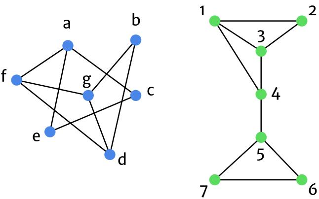
One thing you might say is that they look the “same”, up to the fact that the graphs are coloured differently, and are somewhat rotated with respect to each other. While some may say that these are important distinctions, for the present essay, let’s pretend that this is merely a trivial difference. I think we can agree that these two graphs are essentially the same. Not only do they have the same number of nodes (vertices), there’s a sense that you can “match” up the nodes between the graphs. It’s just like when you were in elementary school and had to find out if two shapes were congruent, similar, or completely different.
But what if I told you that the graph on the left represented the roadways of a small town, and the graph on the right represented a network of people? Suddenly, these graphs don’t seem so similar anymore, practically speaking. And yet, we can still agree that there’s something about their structure that’s the same. What’s great about this is that, if we study properties of the graph dealing with the roads, we can be sure that these same properties carry over to that of the network of people! This seems obvious when looking at the two graphs, because they look just the same, but it’s quite neat that the properties of two completely different kinds of systems can be applied from one to the other.
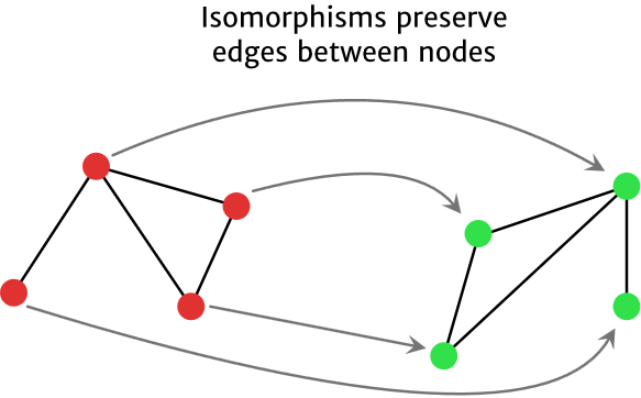
Formally, what I’m talking about in the case above with the two graphs is called an isomorphism. For graphs, this essentially boils down to showing that one can “relabel” the vertices of the graph on the left such that it has the same labels as the graph on the right, while still preserving the same edges between them. If two vertices are joined by an edge in the right graph, then our isomorphism better associate these two vertices in the graph on the left which have an edge joining them.
Isomorphisms are special functions. You can think of them as “sameness” functions. They provide a link between two mathematical objects that show how they can be thought of as two instances of the same thing. I love isomorphisms, because they showcase one of my favourite parts of mathematics: connecting things that seem totally unrelated. In this essay, I want to demonstrate to you the power of isomorphisms. After introducing the concept, we’ll look at an easy example to get a flavour of things, before moving on to the main course.
(Also, can you find an isomorphism for the two graphs? Check the end of the essay for one solution.)
Preserving Structure
As I said above, isomorphisms are special functions. Typically, we denote them as $\phi$, and they are functions from one set $X$ to another set $Y$, with the following properties. First, they are bijective. Another name for this is one-to-one and onto. One-to-one means that any time time you take an element $x$ in $X$ and move it to an element $y$ in $Y$, the only element that gets mapped to $y$ is $x$. Essentially, each element in $X$ gets its own element in $Y$. Then, onto means that any element in $Y$ can be “reached” by using the function $\phi$ on a certain element of $X$. In other words, we have inverses. This is all summarized in the figure below.
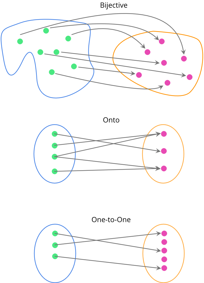
An immediate consequence of a bijection is that the two sets in question have the same cardinality, the number of elements in the set. This is true because each element in $X$ gets sent to an element in $Y$, and nothing in $Y$ is “missed”. That’s a bit of handwaving, but the important point is that these two sets will have the same cardinality if you can establish a bijection between them (which is an exciting topic in and of itself, but will be saved for another time!).
This gives us a bijection between the two sets, but an isomorphism gives us a bit more than that. Not only do we have a direct “link” between the elements in $X$ and $Y$, we also have the fact that the structure of $X$ is preserved in $Y$. If we go back to our example with graphs, not only did we want to send every vertex in the left graph to a unique vertex on the right, but we also want their edges to coincide accordingly.
To encode this mathematically, we want the following property to be true. If $\phi$ is our isomorphism, then if we take $a,b \in X$, $\phi(ab) = \phi(a) \phi(b)$. Let’s untangle this a bit, because the equation is a bit subtle.
On the left hand side, we have $\phi(ab)$. The term $ab$ means you are doing some kind of operation that sticks $a$ and $b$ together. Despite what it may look like here, I’m not only talking about multiplication (it’s just that we usually omit the symbol that signals the operation). The operation could be addition, multiplication, or more exotic things, like turning a number into a complex number, or associating an element with an ordered pair. There are many possibilities (but not all of them are isomorphisms!).
On the right hand side, we have $\phi(a)\phi(b)$. Once again, this means that we are performing an operation between $\phi(a)$ and $\phi(b)$. The crucial part here is that this operation doesn’t need to be the same as the one in $X$. Remember, we are in $Y$ now, so the operation could be different!
Put simply, the idea of $\phi(ab) = \phi(a) \phi(b)$ is that any time we combine two elements in $X$ and then use the isomorphism to go to $Y$, it’s the same thing as going to $Y$ first in each individual element, and then putting them together.
With that out of the way, let’s start looking at some isomorphisms.
Flipping Switches
We’re in no rush, so let’s look at an example that is fairly straightforward. Consider your classic light switch. It can be in two positions. Either the switch is “ON”, or the switch is “OFF”. However, the more important thing is that we have some additional structure on the light switch. There are two things we can do with a light switch. We can “flip” it from one setting to the other, or we can leave it be. Let’s give these operations some names. We will call a flip $\uparrow$, and doing nothing will be called $n$ (for neutral, or “nothing”). Then, we can associate certain operations on the light switches. I’ll use the symbol $*$ to denote doing two operations, one after the other.
First, we can do nothing twice, which results in nothing happening. Therefore, we can say that $n*n = n$. Similarly, we know that if we flip a switch and then do nothing, or do nothing and then flip a switch, the result is that the switch gets flipped once. Therefore, we can encode that mathematically by saying $n \, \,* \uparrow = \, \uparrow* \, \,n = \, \uparrow$. Finally, the last thing we can do is to flip the switch twice, which amounts to the same thing as doing nothing at all. As such, we have $\uparrow * \uparrow = n$.
From these four combinations of operations, we’ve completely specified the structure of our system. Why? Because any more complicated series of moves we can do can be broken down into a combination of these operations. This is nice, because it prevents us from having to deal with many more elements. Indeed, our set of moves we can do on the light switch has only two elements: flipping a switch, and doing nothing.
If we want to be more formal about this, we can call this set with the operation $*$ a group. The way I like to think about a group is that it’s a certain set endowed with an operation that tells us how to “stick” elements together. The structure I was talking about earlier with respect to isomorphisms has to do with this operation. We don’t just have some random elements in a set. We have some way of connecting them together. Furthermore, as we saw in the previous paragraph, no matter how we stuck the elements together, we never formed a new element. We always stayed within our set. This is an important property of the operation that our group has.
Now, let’s look at something completely different. Let’s consider the set of integers under modular two arithmetic. If you’re not familiar with modular arithmetic, the quick summary is this. Modular arithmetic considers what the remainder of all integers are when divided by a certain modulus (integer greater than one). For modular two, we only have the elements $0$ and $1$, because every other integer can be reduced to this by dividing by two until the remainder is $0$ or $1$ (this is equivalent to saying all numbers are even or odd). Therefore, we only have these two elements.
Now, let’s consider what happens if we look at this set ${0,1}$ with the operation of addition. Then, we get the following four combinations:
\[\begin{align}
0+0 \equiv 0 \mod 2, \\
0 + 1 = 1 + 0 \equiv 1 \mod 2, \\
1 + 1 \equiv 0 \mod 2.
\end{align}\]
The first three operations should be clear, but the last one might not be. To see it, remember that $1+1 = 2$. But $2$ is divisible by $2$ with no remainder left over, so it is equivalent to zero.
You might be starting to see where this is going. We’ve just defined two sets with different operations that seem to share a lot of structure in common. They both have two elements, and the way the elements combine together is very similar. So can we find an isomorphism between them? You bet!
Since we are dealing with only two elements in each set, we can specify the function when applied to each element (this wouldn’t be the case if we were working with sets that had many or even infinitely many elements in it). We’ll identify the flip with $1$, and doing nothing as $0$. Therefore, we can write out the isomorphism as such:
\[\begin{align}
\phi(\uparrow) = 1, \\
\phi(n) = 0.
\end{align}\]
Since each element in our set for light switches corresponds to exactly one unique value of $0$ or $1$, we can see that our function is both one-to-one and onto, so it is bijective. What we now want to show is our other property, that $\phi(ab) = \phi(a)\phi(b)$. We will only show one, but the others are just as simple to check. If we take the combination $\uparrow * \, \, n$, we get:
\[\begin{equation}
\phi(\uparrow * \, \, n) = \phi(\uparrow) = 1 = 1+0 = \phi(\uparrow) \phi(n).
\end{equation}\]
As you can see, this works beautifully. Also note that the “operations” for each set aren’t the same thing (one is flipping a switch, and one is doing regular addition), but the structure of the operation gets preserved. Therefore, we’ve got ourselves an isomorphism.
Of course, this is just a simple example (and I’ve left out a few technical details), but I hope it illustrates to you the quite ingenious correspondences we can make between structures.
Let’s go to a bit more complicated example!
Number Systems and Algebra
In secondary school, you’ve most likely studied equations of the form $y=ax + b$, $y=ax^2 +bx + c$, and maybe even $y=ax^3 + bx^2 + cx + d$. There’s even a chance that you remember the name of these functions: polynomials. You probably won’t be surprised to hear that polynomials form a much larger family of functions than you’ve seen in secondary school. Indeed, a general polynomial $p(x)$ can be written as such:
\[\begin{equation}
p(x) = a_0 + a_1 x + a_2 x^2 + \ldots + a_n x^n.
\end{equation}\]
I know that I zone out when I start seeing too many terms on a line, so I’ll try to avoid it as much as possible. However, my point is that any polynomial has this form. We then know how to add and multiply any two polynomials together. For addition, we add the coefficients of the like terms together, and for multiplication, we slowly and painfully multiply everything out and then collect the terms. It might be painful, but it can be done. The important part is that no matter if you add or multiply polynomials together, the result is also a polynomial.
There’s another assumption that barely crosses our minds, but let’s make it explicit. The coefficients for our polynomials will be anything in the reals. This is to distinguish it from other kinds of objects that have coefficients only in the integers, for example. Since our coefficients are real, we will call this set $\mathbb{R}[x]$.
But $\mathbb{R}[x]$ isn’t only a set. Because we established certain kinds of operations on it (namely, adding and multiplying) that result in new polynomials in our set, $\mathbb{R}[x]$ is actually called a ring (and in particular, an integral domain). The name isn’t terribly important, but I think it’s good to be aware of the terms. In essence, being a ring means that the set $\mathbb{R}[x]$ is closed under our two operations, and has a few more technical features.
This is all well and good, but you may be wondering where in the world am I going with this. Where is the isomorphism?
To set this up, remember how we worked in modular two arithmetic, which essentially compressed all numbers into either $0$ or $1$. We’re going to do the same thing here, but with a slightly different flavour. What we’ll do is consider all of the polynomials of the form $p(x) = (1+x^2)f(x)$. In other words, all of the polynomials which have $(1+x^2)$ as a factor. Then, we will that any polynomial with this factor is identified to be zero. Since $f(x)$ can be any polynomial, this means $(1+x^2)=0$, or equivalently, $x^2=-1$. This is really nice, because anytime we see $x^2$ in our polynomials, we can “swap” it for $-1$.
So how does this change $\mathbb{R}[x]$? Remember that all of our polynomials have the form:
\[\begin{equation}
p(x) = a_0 + a_1 x + a_2 x^2 + \ldots + a_n x^n.
\end{equation}\]
We know that the first and second terms won’t be affected, since there are no $x^2$ terms in them. However, every other term in $p(x)$ can be simplified. In fact, since every power of $x$ is either even or odd, any power that is larger than one will be reduced to a power that is less than or equal to one. As such, when we replace all of the $x^2$ in the polynomials with $-1$, we will get a new set of polynomials in the form:
\[\begin{equation}
\{a+bx : a,b \in \mathbb{R}, x^2=-1 \}.
\end{equation}\]
Do you know any other sets with this kind of description? It’s the complex numbers $\mathbb{C}$, of course! The condition that $x^2=-1$ might have given it away, but I think this is just a lovely correspondence that just pops out without you really knowing about it until the end.
The isomorphism now would be of the form $\phi(a+bx) = a+bi$, but this can also be established using the first isomorphism theorem of rings, which we won’t get into here. What I want you to get from this is that we can establish a correspondence between doing some sort of pseudo-modular arithmetic (with a strange modulus) on the set of polynomials, and end up with the complex numbers.
Coda
There are many more isomorphisms, but I think we can call it a day. I love it when we can find correspondences between objects that somehow capture a notion of being the “same”, yet still seem different. It’s when we view them from a different perspective that we see that there differences aren’t really fundamental.
Lastly, the solution to the problem I posed at the beginning of the essay. The isomorphism between the graphs is given by the following. Send vertex $a$ to $5$, $b$ to $2$, $c$ to $6$, $d$ to $1$, $e$ to $7$, $f$ to $4$, and $g$ to $3$. The way I look at the problem is to imagine trying to find a way to twist and bend one graph into the other. However, this only works when you know that there is an isomorphism beforehand!