The SATisfying Physics of Phase Transitions
For the past few months, I’ve been thinking about the following equation.
Specifically, I’ve been wondering about the possible configurations that solve this system of equations.
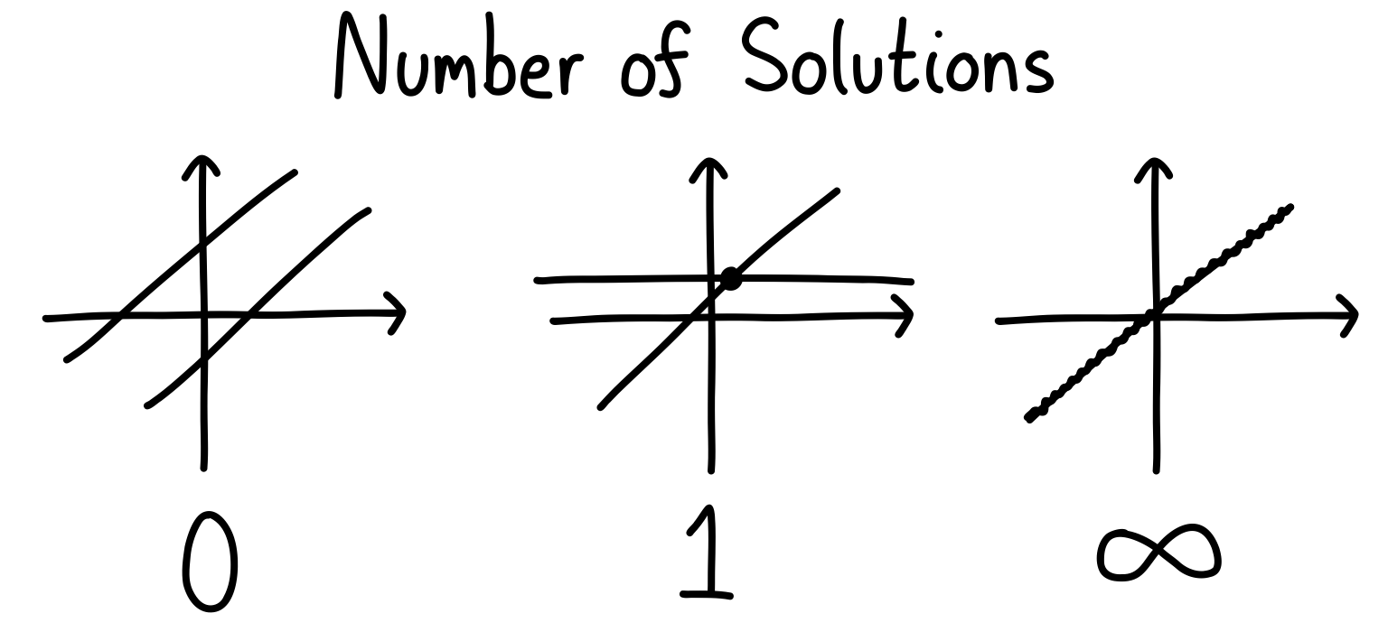
If you’ve taken a linear algebra course, you will remember (okay, maybe you will remember) that this equation can have no solutions, one solution, or even infinitely many solutions. To get a handle on these three cases, think about a system of equations of two variables. We can plot the cases as lines in the plane (let’s imagine we only have two equations for now).
If we want to apply an algorithm to find the number of solutions, the way to go is with Gaussian elimination. This is perhaps the most practical thing you learn in a linear algebra class, but of course it’s not something that you should be doing by hand. Instead, we can write some code so that any matrix we feed in will give us this information.
Okay, I didn’t tell you the full story.
While I have been thinking about the above equation, I’ve neglected to append an important part to it. Instead, the equation I’ve been thinking about is: The rules for manipulating equations and matrices are the same, but the difference is that now we’re working over the binary field. That’s a fancy way of saying that algebraic manipulations obey: Plus, any time we have a number, we’re allowed to divide it by two and take its remainder. So and . Essentially, this encodes whether the number you’re dealing with is even or odd.
In the binary field, we don’t have to worry about negative numbers because these can always be converted to either zero or one. In fact, everything we deal with will either be zero or one. So no fractions, no irrational numbers. Only ones and zeros.
This simplifies things quite a bit, but still leaves us enough structure to have some fun.
Instead of having finitely many or infinitely many solutions, we now only have finitely many (including zero). The nature of modular arithmetic and only using zeros and ones means we’ve reined in that pesky infinity.
The number of possible solutions can be calculated directly. Because we’re dealing with binary entries in all of our objects, our vector will have exactly possible configurations, where is the number of variables (each component has two choices, so you get ).
To recap, we start with the equation: The matrix is an binary matrix, is an -component binary vector, and is an -component binary vector.
Then, we’re going to ask the following question:
What happens to the solution space on average as we increase ?
This question will carry us from linear algebra, to theoretical computer science, and finally to statistical physics.
Ensembles
When posed any question that uses the word average, you should reply, “What ensemble are you using?”
Seriously, the ensemble you choose determines everything. Imagine I told you that the average person loves running 100+ kilometres every week. This would probably seem pretty strange. Except the people I asked were all long-distance runners who have been doing this for years.
The ensemble I chose (experienced long-distance runners) informed the sort of average I would then calculate.
In the exact same way, if we want to answer a question probabilistically in mathematics, we should be careful about our assumptions and how we define our ensemble.
Here’s a recipe for drawing a sample from an ensemble:
- Choose the number of variables .
- For each row, choose three columns to contain a one, and set the rest to zero.
- Repeat for the rows.
- Choose the components of the vector at random from .
- If any row is repeated, resample until it’s different.
After this procedure, you will find yourself with a matrix and a vector . You can then plug this into your favourite tool to solve binary matrix equations, and see what comes out!
Before we start averaging, let’s think about what an equation will do to the configuration space.
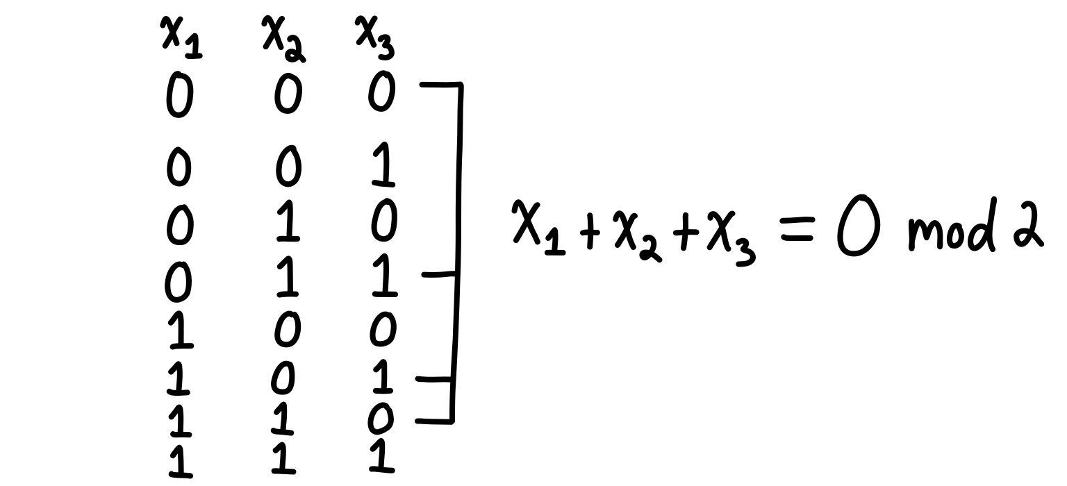
At first, we have no equations, so every configuration is a solution. As we saw before, there are of them. After we insert one constraint (a row of ), this will specify the parity of the sum of three variables. It doesn’t matter what variables we look at, or how many of them. The parity can be odd or even, so half of the configurations will remain, and the other half are tossed out. The diagram below shows how imposing the parity to be zero selects four configurations, leaving the other four to be discarded.
This happens only when is small. However, as you make larger, there are more rows of the matrix which can “interact”. In the language of linear algebra, the rows will eventually become linearly dependent, at which point the solution space will stop being chopped in half for each extra row, but will decay more slowly.
Different Disguises
I began this essay by talking about linear algebra, but this problem pops up in many different fields of science.
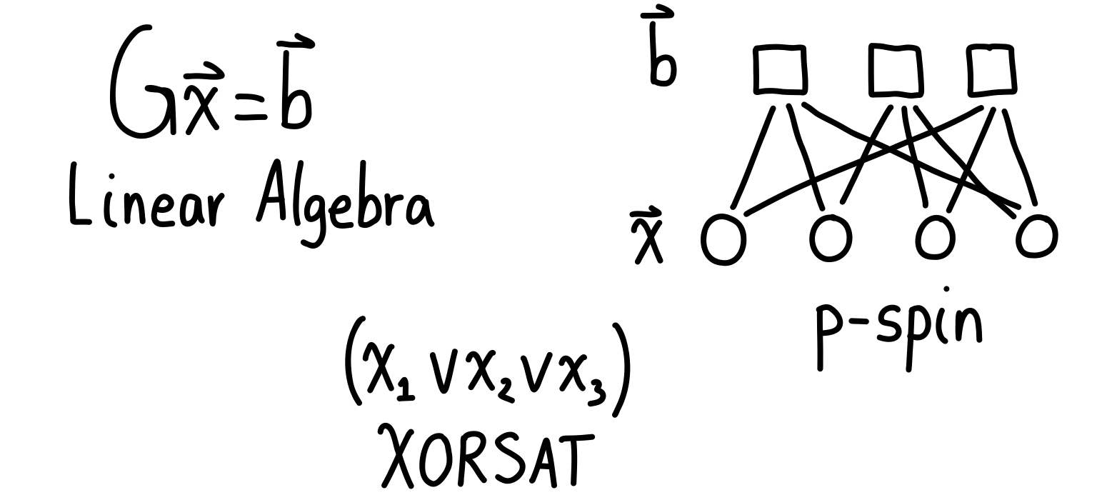
In theoretical computer science, this goes under the name of -XORSAT, where in our case. This is a satisfiability problem, which means you have a bunch of variables (the vector from above) and then you have constraints (the matrix along with the parity vector ), and the question is if you can find a solution to the problem. Answering this is then the same as performing Gaussian elimination and determining if a solution exists.
In statistical physics, we call it the -spin model, where in this case. Instead of a binary variables, we map them to , which are the values of the particles’ spins. For any variable , the spin variable is . The matrix tells us how the particles interact (the constraints), and the vector is the spin configuration of the system. We can then define a Hamiltonian (think of this as an energy function), which has its lowest energy when all interactions are satisfied. Finding a solution to in the -spin language is about finding a ground state of the system.
The Phase Transition
Hopefully you’ve thought about what happens to the presence of solutions as we increase . Actually, it’s better to talk about the parameter , since this takes into account how big the system is (the larger the number of variables, the more equations you should be able to add before completely constraining everything). Once we’ve done this, we can ask what the probability of having a solution looks like as a function of . And when I say the word “probability”, I’m thinking of looking at many samples of a matrix and parity vector , and then averaging.
Here’s what it looks like, as an animation:
It’s a drastic change. Either you will certainly have a solution, or you won’t. There’s a very brief transition period where the probability goes from one to zero, but this becomes smaller and smaller as .
To me, I can’t help but yearn for an explanation for why this is happening.
Here’s one perspective. As you add more and more vectors (rows) to your matrix , there will come a point where some of these rows will become linearly dependent. At this point, the values of the parities for these rows will become super important. If they aren’t set the right way, there will be no solution (since there will be a contradiction that can’t be resolved). And since is chosen uniformly at random, there will often be no solution. Average this over a bunch of matrices, and you will get a curve like the animation above.
Where should this happen? An upper bound that seems reasonable to me is , since that is where a matrix can become full rank, and therefore adding more rows makes them linearly dependent. However, since we’ll likely start having dependent rows sooner, the threshold will be lower than that.
There’s also a perspective related to graph theory. It has to do with a notion of hyperloops, but this will take us a bit further than I want to go. If you want to learn more about it, see Endnote 1.
But here’s the catch: If we change the equation to , we still get a phase transition like the one above. The difference is that now the number of solutions is always at least one (since is always a solution), so the transition is picked up with a different measure.
And that measure is found by taking the statistical physics perspective.
Who Ordered That?
Order, symmetries, and large-scale structures are the bread and butter of statistical physics. We want to go away with the pesky details, and instead focus on the big picture.
The concept of magnetization is one way to measure something about the system as a whole. Like a person who just learned about hammers and now sees everything as a nail, magnetization is used in many contexts. But at its heart, magnetization is a way to measure similarity.
Imagine we have a bunch of particles which can take spin values of , where is just the label for a particle.
Many models we have in physics have rules that ask for the spins to align. These often go by the name of Ising models, and they are the iconic models for statistical physics. The Ising model usually involves some system of spins, with neighbouring interactions. The spins “want” to align, but when the temperature of the system is high, they have energy to not align. In fact, the spins will basically be distributed randomly. In two-dimensions, the model undergoes a phase transition as you lower the temperature. The spins go from being randomly distributed to being either all pointing up () or down (). This happens at a critical temperature called .
The measure we can look at here is the magnetization of a sample, which is just the average of the spin values: If , this means the spins are all aligned (either up or down). Whereas if , then there are an equal number of spins that are up and down.
For an absolutely marvelous discussion about magnetization (with beautiful animations), I highly, highly, highly recommend Brian Hayes’s latest essay, “Three Months in Monte Carlo”. If you look at Figure 2, you will see the phase transition as a function of the temperature. I’ve drawn what it looks like below.
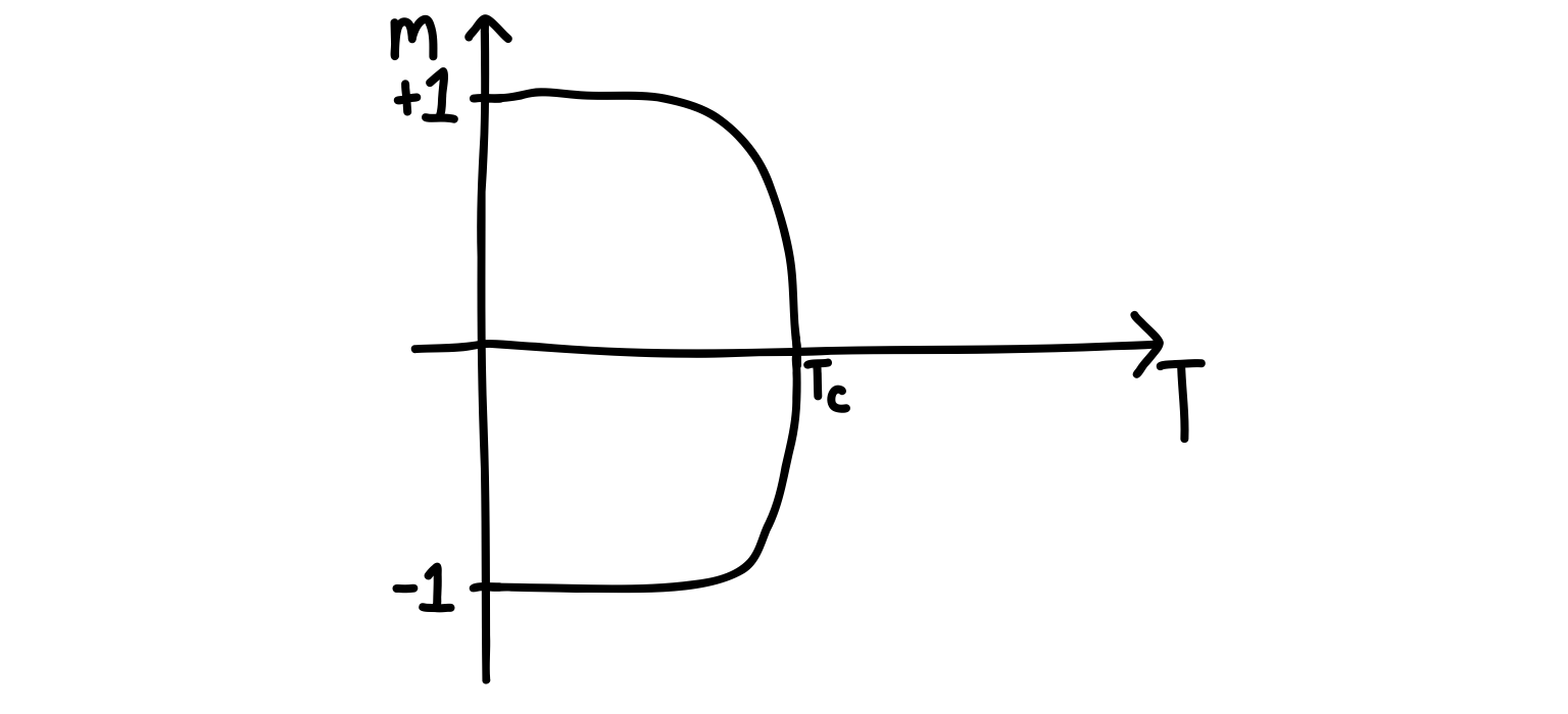
We need to be careful when interpreting this diagram. It’s what happens for one sample of an Ising model. As you decrease the temperature, the sample will “decide” to either go towards or . This happens differently depending on the particular random details of a sample. The problem is that if you start averaging your value of over many samples, you will find the whole curve is flat at . This happens because the samples going to as we cool the system will cancel each other out in the averaging.
Combatting this is straightforward: Instead of plotting , we can plot or . Just keep this in mind if you’re trying to implement a simulation like this in code and are getting confused as to why you don’t see the transition.
Let’s take a look at how the magnetization changes as we increase .
It turns out that for our purposes, plotting just is fine. However, because of a technical aspect of the sampling, it will be better to plot something slightly different: This is called the spin glass order parameter (see Endnote 2). There are a few layers of abstraction here, so let’s break them down.
The square brackets are used to find the magnetization per site. Concretely, they indicate an average taken over the same site for different solutions to the equation . This result will always be between .
If you get a result of , this indicates that all configurations have the same value for this variable. On the other hand, tells us that there is no tendency for variable to be either value.
So while there are three values that describe the “extremes”, really there are two extremes: every configuration takes the same value for a given variable, or there is no preference.
To capture this numerically, we can simply square the result. If there is no tendency for a variable to be one value or the other, this will still be true after squaring. But now we won’t discriminate between variables which have been “magnetized” to versus .
The average in angular brackets now tells us to average this overlap quantity over all the variables. This makes it super simple for plotting purposes, since we have just one number. However, you could forego the final average and just plot the average spin-glass order parameter as a probability distribution over the different variables (giving you a histogram-like result).
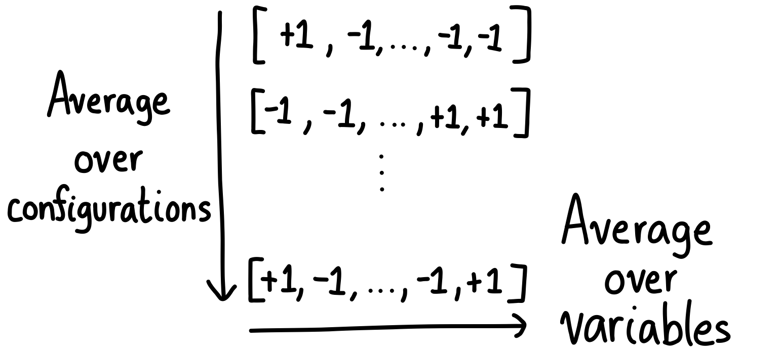
To recap, there are three averages being done:
- An average over configurations.
- An average over variables.
- An average over samples.
If you picture these configurations as arrays, it looks like this for a given sample:
When calculating the order parameter, we have to look at many matrices for the curve to smoothen out like in the animation. (I promise we’re now done with the averaging!)
If you carry all these steps out, then you will be rewarded with a beautiful plot like this.
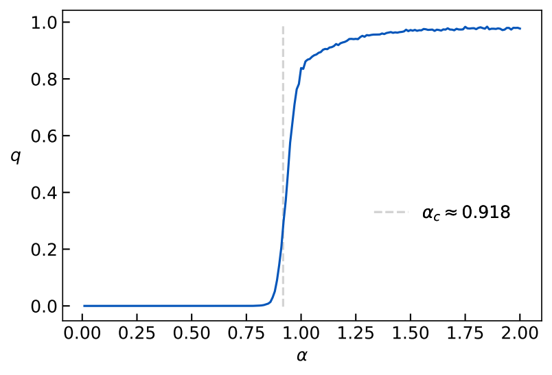
And there’s the transition! So the order parameter picks this up quite nicely. (Note that this is for , )
After the critical threshold , the variables all become magnetized, gravitating towards the solution . The interpretation of the transition is the following: All of the remaining solutions after the threshold “cluster” around the solution .
Where exactly is the transition located? It turns out to be approximately at , which is the in specific case of for our model. I won’t go through the details of how to find it here, but check the References for the paper that shows this.
Clustering
To get a feel for the transition, I wanted to make an animation focusing on one specific sample. It’s a 900-variable model, and I’ve arranged it in a 30x30 square for convenience. Don’t take too much stock in the arrangement of the variables, which are shown as squares. Remember, the interactions can occur between any three of the variables, so this is just for show. I’m plotting the order parameter at each site, which is the same as the equation for the order parameter without the final averaging over all the sites (the angular brackets). Watch for transition, which occurs at .
Dramatic, no?
Notice how the variables are mostly undecided between values, indicated by their lighter colour. However, as we approach the critical threshold, there is suddenly an influx of darker squares, and it soon takes over the board.
Watching this is very satisfying. It gives me a sense of what’s happening in the transition, with each site being free to do whatever it once until the threshold is reached. At that point, there is a force pushing all of the variables to match each other between configurations, until we have only one solution left. (There are still multiple solutions in the animation above, since not all squares become dark. This is because I didn’t go to a higher value of .)
When you keep adding more rows to your matrix , the moral of the story is that you will eventually reach a critical point where all of the solutions have the same values for most of the variables.
Satisfiability
This is just the tip of the iceberg when it comes to satisfiability problems. These are problems with constraints and a vector that attempts to satisfy them.
The setting of -XORSAT is nice because we can do large simulations through Gaussian elimination, which is an efficient algorithm. In fact, the existence of Gaussian elimination is what makes -XORSAT a problem that’s in the complexity class P. Many other satisfiability problems are in NP, but they often show the same sort of phase transition. Since we can analytically wrap our heads around -XORSAT though, I figured this would be a good starting point for the curious learner. Plus, the statistical physics version of the model is easy to think about, making it an attractive starting point.
What began as a simple question about solutions to a matrix equation lead to a discussion about statistical physics, magnetization, and the nature of Gaussian elimination. The phase transition tells us something really specific about the average behaviour of these systems. You may have thought that all matrices are their own beasts, but it turns out that they can be remarkably similar in their behaviour. The perspective of phase transitions teaches us that abstracting away from the particulars can lead us to simple explanations of complex phenomena.
Thank you to Grant Sanderson of 3Blue1Brown, James Schloss of LeiosOS, and everyone else who made the Summer of Math Exposition happen! All of us in the community appreciate what you’ve done.
Endnotes
- The notion of hyperloops and how they affect the -spin model can be found in Section V of this paper. I will warn you though: the diagrams are so old that they are very bad. Honestly, understanding the notion of a hyperloop gave me a headache looking at Figure 1. I might have to write an essay on this idea just to give people a better introduction!
- The spin glass order parameter is not consistently defined if you scour the literature. The idea is to have something that captures the overlap of different solutions (sometimes called replicas). You can look at only two replicas, or many. Here I used many, but the effect is robust with two (though it takes more samples to get the curve to smooth out for the averaging).
- Some technical tidbits. Because the number of solutions is exponential in , I couldn’t do the full averaging over solutions that would be required for the animations and plots. Instead, I made a compromise. I set the number of sampled solutions to be the minimum between 100 and the number of remaining solutions. This mean that I would look at 100 configurations for every matrix at a given , unless the total number of solutions was fewer than this, in which case I took them all. This makes things a bit more memory efficient, and shouldn’t affect the results much.
References
- I already mentioned Brian Hayes’s essay “Three Months in Monte Carlo”, but I would recommend all of his essays on Bit-Player if you’re the type of person who loves reading about computation.
- A recent two-part blog post on the theory of replicas can be found here on the wonderful blog Windows on Theory. In the post I’ve linked to, they briefly discuss the satisfiability phase transition, as well as work out some of the pesky integrals needed to analyze the behaviour of these ensembles. The post is about machine learning, so this gives you an idea of how broad these ideas are!
- The paper “Alternative solutions to diluted p-spin models and XORSAT problems” gives a more theory-based overview of what I covered in this essay. In particular, the paper shows how to derive the threshold by finding the solution to a transcendental equation (in the paper, it’s Equation 42).