As a quantum theorist, my job is to study quantum systems and understand their inner workings. However, since I’m a theoretical physicist and not a experimental physicist, most of my “experiments” come in the form of simulations. My laboratory is my computer, and this means writing numerical experiments.
But wait a second, you tell me. Isn’t the whole point of quantum computers to do things that our regular computers can’t? And aren’t there issues with exponential memory?
These are both very good questions, and we’ll dive into them below. But in short: Yes, these are issues that limit the experiments I can do. And it’s a reason I’d like to get my hands on a good, error-correcting quantum computer!
In the absence of one, I make do with classical simulations. However, depending on the job you want to do, different techniques are preferable. Since I’ve begun my PhD, I’ve learned how to simulate quantum systems using a variety of techniques. Each has their own quirks, and for someone as code-averse as I was, I’m happy to say that I’ve slowly found my groove.
The thing I’ve learned through all of these methods though is that simulating a system (any kind of system) is often very different from the actual system itself. When I write a simulation, what I’m trying to do is map the system I want to study to objects in my code which I can handle more easily. To put it concretely: While I imagine my “simulation” of qubits to be some strange quantum system, the reality is that it’s a bunch of lists and arrays being transformed using the tools of linear algebra.
At first, this really bugged me. After all, I want to simulate my quantum system, but what I’m really spending my time on is converting it into a language my computer can understand. These layers of abstraction between the system that I want to simulate and its representation in a computer is something I’ve learned to deal with. In a way, writing a good simulation is an art form in and of itself, since you have to figure out an equivalent way to represent your system as code.
As you will see, there are many ways to simulate quantum systems now, and each one has its own representation. Therefore, if you want maximal control over your simulation, it’s a good idea to learn the techniques required. There is a point in which you should just say, “Okay, I don’t need to know how this underlying thing works,” but I think this point is further than I used to believe.
Finally, working with numerical simulations has taught me something very important about mathematics: It’s one thing to see an equation in a paper. It’s a whole other thing to implement it in code and see it give you results. Often, an equation hides a lot of numerical baggage which needs to be implemented before you get a result. As my friend said in a presentation, “You don’t understand X unless you’ve coded it yourself.” This is something I’ve heard from others as well, and I think there’s a lot of truth to that statement. Which is why I try not to shy away from learning new coding practices when it comes to my research.
This essay will be broken up into three categories, which roughly describe the kinds of methods for simulating quantum systems that I’ve worked on. I’ll mention the specific libraries and tools I’ve used, but the point here is to discuss the broad categories, since those are more important than the specific tool.
State Vector Simulators
This is probably the “closest” simulator to the kind you would imagine in reality. What I mean by this is that you start with your quantum state $\vert\psi\rangle$ and it evolves according to various quantum gates that apply on your system.
Schematically, the evolution looks like this:
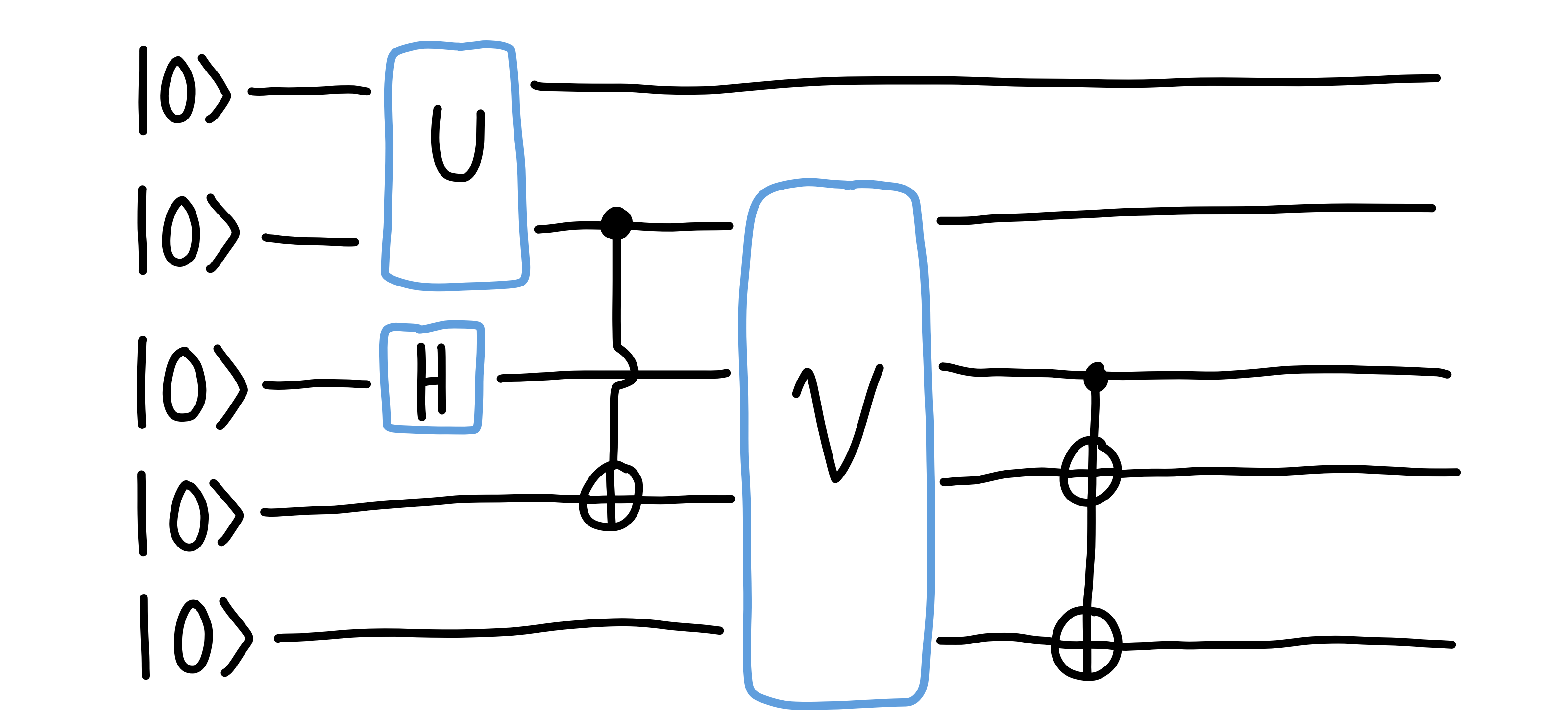
In other words, you start with an initial quantum state, and each gate you apply is a unitary matrix which multiplies your initial state. So if I apply some quantum gate $U$ on my system, the resulting state is $U\vert\psi\rangle$.
One thing you might notice is that a circuit which is drawn left-to-right (in the sense that the initial state is on the left) is written in the reverse way when seen as matrix multiplication.
For me, the state vector picture is the easiest way to work with a quantum experiment. I just have to define my gates (the usual suspects like the Pauli operators and the CNOT gates are already defined), and then specify how they apply to a specific qubit. The libraries which do this sort of simulation then take care of actually building the right matrix $U$ to apply to the system.
The main library I’ve used here is Qiskit, because of the above-mentioned partnership we have with IBM.
A very important point I want to make here is how this underlying matrix $U$ is built. Let’s say we have three qubits, and we want to apply an X gate on the second qubit. As an operator, it would look like this:
\(U = 1 \otimes X \otimes 1.\)
This is fine as a notation, but as a matrix, it becomes 8×8, which is starting to get big. In fact, if you have N qubits, then each individual qubit matrix is 2×2, so in total the size of the resulting matrix $U$ is 2N×2N. As you can probably imagine, this doesn’t scale too well for large system sizes.
At the end of the day, the reason this isn’t sustainable is because the vector needed to describe quantum state has 2N components for N qubits. That’s fine for small systems, but if we want to start making claims in the “thermodynamic limit” of some quantum system when N→∞, we quickly get stuck.
So the state vector picture is a nice starting point because there’s a very direct connection to what’s going on. The elements you see in the circuit are matrices, and they keep on multiplying the initial quantum state until you get to the end. There are a few more subtleties when it comes to measurements, but that’s the gist.
The drawback is that you can’t scale up very high in the circuit picture. To give you a rough estimate, in Qiskit’s online version of their statevector simulator (this directly deals with the quantum state) and the QASM simulator (more for dealing with measurement results), their upper limit is 32 qubits. I think you can potentially go higher on your own hardware if you have enough RAM, but when I say “higher” I mean something like two extra qubits. Again, this has to do with the exponential cost of storing a quantum state. Each new qubit requires double the information to store. This is the crux of the bottleneck, since doing linear algebra with a big object like that is not easy.
But what if you didn’t need all those components? What if some of them you knew were always zero, or some were fixed by a property of your system? Then, is it possible to shrink the amount of space needed to simulate a circuit?
The answer is yes, and this brings us to tensor networks.
Tensor Network Simulators
The term “tensor network” feels like a buzzword to me in a similar manner that “machine learning” does. To me, these two words just sound cool, and make it seem like a lot of neat research can be done with them.
In fact, saying this section is about tensor networks is like saying this essay is about quantum theory. Sure, but that’s pretty vague. There are a bunch of different areas of tensor network research, but the one I’ll be focusing on here deals with a representation of quantum states called “matrix product states” (MPS).
People are really good at naming things, so it turns out that the main object of an MPS is not a matrix, but a tensor. I plan on getting into tensor networks much more in future essays (because this is related to a lot of my research), but here are the essential bits.
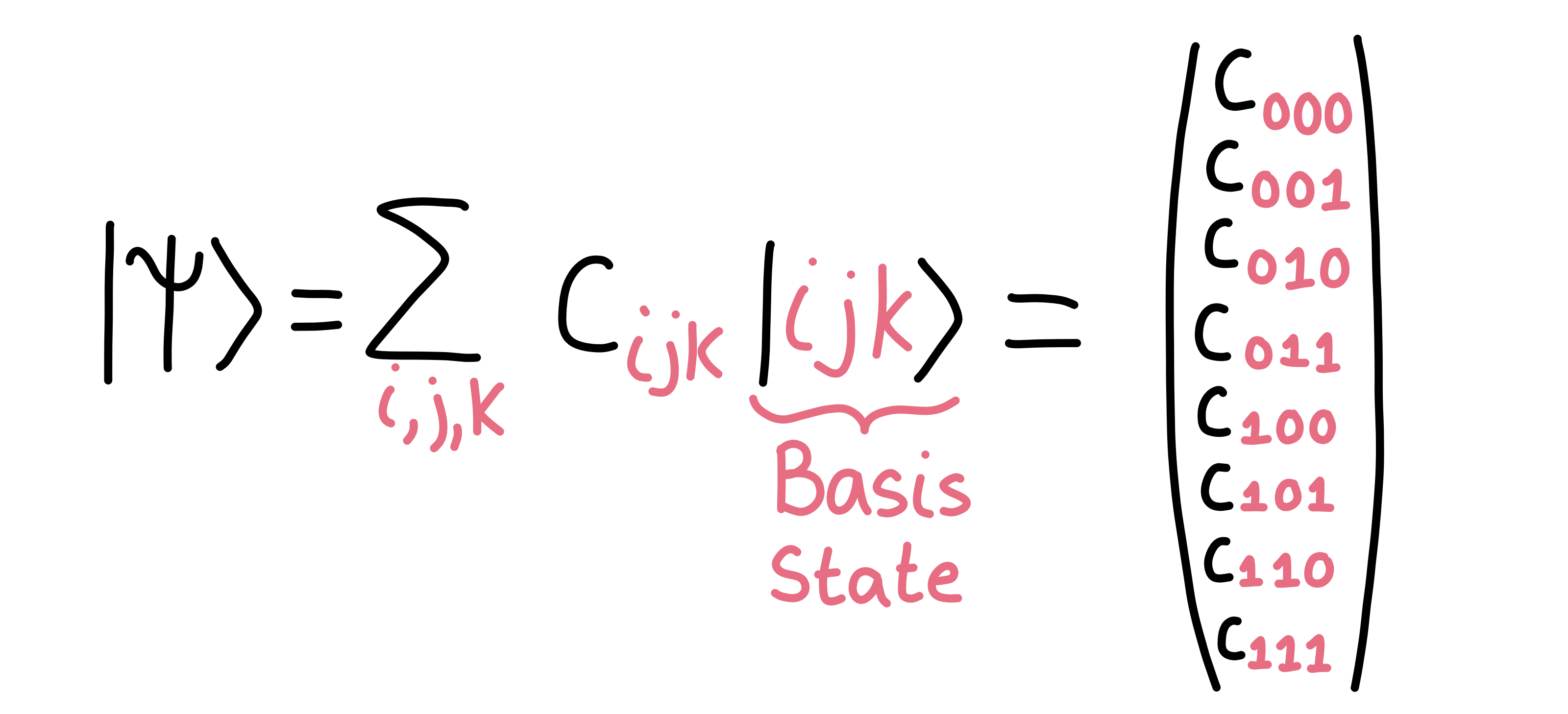
When you have your quantum state $\vert \psi\rangle$, you have to keep track of all 2N components. In fact, if we want to write things out fully, we can write down our quantum state (over three qubits, for example) as:
\(\vert \psi\rangle = \sum_{i,j,k} c_{ijk} \vert ijk\rangle.\)
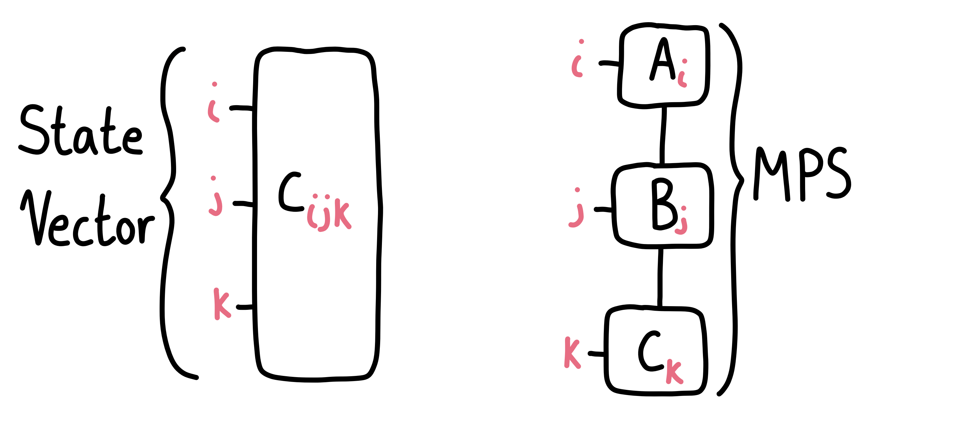
The coefficients $c_{ijk}$ are precisely all of the different entries of the state, and the vector $\vert ijk\rangle$ is the basis state, which tells us where to put the coefficient in our state $\vert \psi\rangle$. As a diagram, we can think of it like this:
The MPS form of a quantum state is a way to split the coefficients $c_{ijk}$ such that they are each defined on a single qubit. This doesn’t come for free though, so what we end up doing is creating tensors that can be chained together to reproduce the coefficient $c_{ijk}$ if we multiply everything out. I won’t show you all of the indices in this essay because it would scare you off (a future essay should cover it), but as a diagram, here’s the idea:
With this, we can potentially save space on the number of elements we need to store (see Reference 1 for more). In my case, using the MPS form of a quantum state allows me to study the entanglement entropy of a quantum state while never having the full 2N object in memory. This allows for more qubits to be simulated. For example, Qiskit has a MPS backend, and you can go up to 100 qubits with it.
The downside is that you can’t do anything that builds the whole state vector. For example, you can’t check what the full quantum state is, only what it is in its “decomposed” form. You can think of it like this: We’ve broken up a huge quantum state into a bunch of small packages which we can handle. What we can’t handle is putting them all back together.
Applying gates to an MPS is conceptually straightforward but I found it was difficult to get it working in code. That’s because you need to take care of so many indices. In a sense, it’s “just” multi-dimensional linear algebra, but that “just” is doing a lot of work.
What’s nice though about applying gates is that you can apply them without the operator becoming too “big”. They only apply to a single site (or perhaps a few sites) at a time, which reduces their size.
There are costs to this method though. The main one is that you need to do a ton of singular value decompositions, and this becomes expensive as you have more and more qubits arrange in a line. There are alternative ways to deal with this, but I’m not as familiar with them.
Clifford Circuit Simulators
The final method I’ve learned how to do involves very particular gates called “Clifford” gates. Quantum circuits that are built up of only these gates, which are the CNOT, SWAP, Pauli X, Y, Z, the phase gate P, and the Hadamard gate H, are special. That’s because we can drastically reduce the number of objects we need to store in memory when simulating these circuits.
Usually, we want to keep track of 2N components (or perhaps somewhat less if we’re using tensor networks), which grows quickly. But in the case of Clifford circuits, the number of objects we need to track only grows linearly with N.
How can this be?
It has to do with the fact that we can represent quantum states in Clifford circuits using what are called “stabilizer generators”. If you’re a long-time reader, you may remember I covered stabilizers in “A Game of Loops”, where the stabilizers were the plaquette operators acting on my surface code. Using this, I was able to think of my quantum state’s evolution mainly through these operators (though in that case I also looked at the full 2N objects).
I won’t go through all the technical details of the stabilizer formalism here, but the gist is that we can represent quantum states using a set of operators which “stabilize” the system, and do evolution by evolving these objects. See Reference 2 for more on this formalism.
This means that if we have a stabilizer G acting on the quantum state, then G essentially acts as the identity. It’s not the identity, but the combined action of the operator on the quantum state looks like an identity operation.
To give you a small example, imagine we start the quantum state in the computational basis state $\vert \psi\rangle = \vert 00110\rangle$. It turns out that there are precisely five stabilizer generators which stabilize the state (apart from the identity). They are:
\(Z\otimes1\otimes1\otimes1\otimes1, \\
1\otimes Z\otimes1\otimes1\otimes1, \\
1\otimes1\otimes -Z\otimes1\otimes1, \\
1\otimes1\otimes1\otimes -Z\otimes1, \\
1\otimes1\otimes1\otimes1\otimes Z.\)
You can check that applying these operators to the quantum state results in no net change. And using some principles of group theory, it turns out that these can generate any sort of other stabilizer we might dream up, such as $1\otimes1\otimes Z\otimes Z\otimes1$, which is a combination of the third and fourth generators above.
So this is great for representing a quantum state, but the real magic is that this representation gives us a way to simulate the evolution of a quantum state.
That’s because a stabilizer state will remain a stabilizer state as you evolve it in a Clifford circuit. The only difference is that the generators will change. To evolve a quantum state then, all we have to do is track how these generators change (and remember, there are only N of them).
For example, suppose we apply a Hadamard gate on the first qubit. This gives us the transformation $H\vert 0\rangle = \vert +\rangle$, so our new quantum state is $\vert +0110\rangle$. We then change the stabilizer generators to account for this, and we end up finding:
\(X\otimes1\otimes1\otimes1\otimes1, \\
1\otimes Z\otimes1\otimes1\otimes1, \\
1\otimes1\otimes -Z\otimes1\otimes1, \\
1\otimes1\otimes1\otimes -Z\otimes1, \\
1\otimes1\otimes1\otimes1\otimes Z.\)
The rules for changing the generators can be found in Reference 2. I won’t go through all of them here, but there are tools that track these changes automatically, and all you have to do is supply the quantum circuit. The idea here is that these generators can be represented by a binary matrix of size N×2N, where N is the number of qubits. There are 2N columns because we will essentially keep track of the X and Z operators separately. These are all we need to specify our state, and so each one will get its own N×N matrix. Within this binary matrix, a 1 tells us that there’s a Pauli X or Z at the given site. Then, simulating the circuit requires updating this matrix.
Personally, I haven’t created my own simulator. The one I’ve used is called Stim, by Craig Gidney. It’s fast, it works for my purposes, and I don’t have to reinvent the wheel. There’s also a Clifford circuit simulator in Qiskit, where the online version says it can simulate up to 5000 qubits. I’ve used Stim to simulate circuits with about 3000 qubits, so I can attest that this is achievable (though I was using a supercomputer). Now that I think of it though, the longest part of my computation was probably what I did after simulating the circuit and getting this matrix. The linear algebra on such a matrix becomes quite long.
Using this formalism is fantastic if you want to simulate really big system sizes. Unfortunately, it also depends on what you want to study. For example, it’s possible to use these Clifford circuits to get the entanglement entropy, but it’s not possible (as far as I know) to get the entanglement spectrum (the eigenvalues of the reduced density matrix for a state) using this method. So depending on what you want to study, this might not be helpful.
During this first year of my PhD, I’ve been in a sort of transition mode. I’ve had to learn the ropes in both this field of quantum system, as well as how to work with code and numerical tools. The learning curve has been high at times, but I’ve found an appreciation for building my own tools that are perfect for my needs.
I came across a blog post on exactly this by Matthew von Hippel. As a lazy person, I love being able to just grab some code off the shelf that works for my needs. But as a scientist, I know that it’s probably a good idea to build up a set of tools that I’m confident will work. This isn’t easy, and it often involves a lot of “wasted” time where research isn’t moving forward as quickly as I want. But once I have the tools built, I can then tweak things to my heart’s content.
In my case, this has been a year of learning techniques on how to simulate quantum circuits. Learning the ropes of the three methods above has been a big part of my research, and I’ve reached the point where I have a decent enough handle on these aspects that I can use them to start answering questions.
I hope to write more about how these tools are used in my research in future essays. For now though, I’ve built my toolbox, and now I can start digging into the research.
References
- I really like the this site, which explains the various ways to use tensor networks to simulate quantum systems. In particular, the MPS article, is well-done, and the link I’ve provided here will give you an idea for how many parameters you need to describe your MPS.
- The Clifford stabilizer formalism for simulating quantum circuits was developed (to my knowledge) by Scott Aaronson and Daniel Gottesman in this paper. There are others as well around the same time using slightly different approaches, but this is the one I’ve based my code on.
Endnotes