If I ask you what comes to mind when you think of physics, what would you answer?
Stars? Galaxies? Black holes? Particle colliders?
For better or worse, some fields in physics have taken up more of the limelight than others. The astrophysics-oriented answers are the ones my family would likely default to if asked about physics. And I don’t blame them: astrophysics is a branding master.
In fact, studying the universe was the first field of physics that I thought I would study. It seemed like the perfect fit for me, and I eagerly did multiple research internships over the summer with my supervisor Valerio Faraoni (who is great!). I got to study general relativity, think about extensions to the field equations, and dove into a lot of heavy mathematics.
While it was fascinating, I couldn’t help but feel like I was missing something. The physics I was learning didn’t seem tangible to me. It was difficult to grasp it and wrap my head around the problems I was studying. When I went to Perimeter for my Master’s degree, I made sure to try something new.
That something new was condensed matter and statistical physics. As an undergraduate, I wasn’t exposed to these fields (apart from a few thermodynamics courses). I soon learned that condensed matter offers a whole world of physics that I had never encountered before (see the References).
To me, condensed matter is about studying the behaviour of systems of building blocks. These building blocks vary from scenario to scenario, but physicists like to pin down the sort of collective (or emergent) behaviour that occurs when you have a bunch of these building blocks interacting.
(As a side note, statistical physics is often used in conjunction with condensed matter. The main distinction in my view is that statistical physics can be applied to all sorts of building blocks, while condensed matter tends to use particles as its building blocks. Statistical physicists might study the flow of traffic in a congested city, while condensed matter physicists might study the flow of electrons in a material.)
What I love about condensed matter and statistical physics is the way I can get a handle on what’s happening. To study a system, you first establish the building blocks and the rules of the game. Then, you ask questions about the collective behaviour of the system.
While it’s not easy to picture what’s happening when the number of building blocks into the hundreds and thousands, the rules of the game are often simple enough that thinking about a small example in your mind is doable. Even better, you can program an animation to see things in action! This can give you a glimpse of processes that just won’t jump out at you from the equations.
At the end of the day, numerical simulations and mathematical analysis are how we study these systems. However, I can’t express how critical it is to me to be able to picture the system I’m studying in my mind’s eye. Does this help the analysis? Not really. Does it give me another way to pose questions and think about directions that aren’t obvious in the mathematics? Absolutely.
However, it turns out that if my family would start saying I study condensed matter physics, they would still be slightly off.
Graphs and Optimization
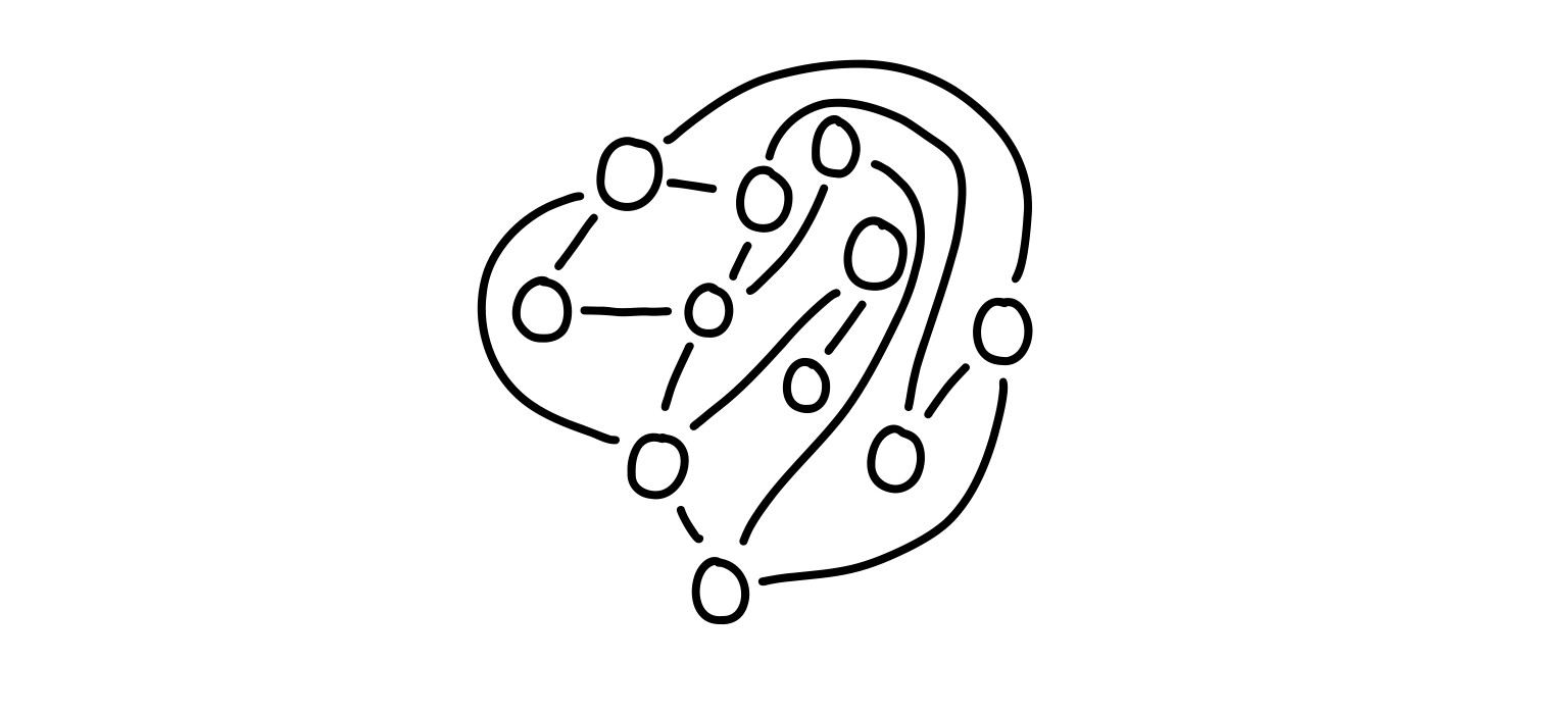
The building blocks I play with aren’t particles or cars in a city, but graphs. These are objects which consist of nodes and edges that connect them. Think of a map, and place a node on every city while connecting those that have roads that go from one to the other. The resulting object is a graph. A graph is a representation, so it can be used in a bunch of different situations.
The rules of the game involve the edges, and usually a notion of giving values or colours to the nodes. For example, imagine I give you the following graph and ask you to use as few colours as you need to colour the nodes. The only restriction is that no adjacent nodes (they are connected by an edge) can have the same colour.
For the above graph, after some trial and error you might find that it can be done with only two colours.

Like I mentioned before, the rules of the game are pretty simple. You have a graph, and you need to colour the nodes. Easy.
But if I give you the following graph, things get trickier.

The rules are the same, but the connectivity of the graph makes things more difficult (for those that are curious, this is called the “Petersen graph”, and can be coloured using only three colours). Even though the number of nodes is actually less than the previous example, it might be trickier to find a solution. What we need is a more systematic way to tackle this problem. One that can preferably be programmed on a computer.
This problem (and many others like it) are called combinatorial optimization problems. It’s “combinatorial” because of how the configuration space (in our case, ways to colour the nodes) grows as a function of the system size. If you have ten shirts, three pairs of pants, and five pairs of shoes, the total number of outfits you can rock is: 10 × 3 × 5 = 150. It’s this kind of growth which brings about the name “combinatorial”.
When I write “optimization”, I’m referring to the fact that we want to solve our problem subject to some constraints. In the graph colouring problem I gave above, a way to solve any such problem is to use N colours, where N is the number of nodes. That way, each one will be distinct, and so we’re done.
We want to do better than that. For the solution of the first problem I gave, while you can definitely colour it with N = 11 colours, two is enough. In a sense, using two colours is the more “economical” way of doing things.
Optimization tends to mean maximizing or minimizing some quantity. In the graph colouring case, our goal is to colour the graph with our rules, while also using as few colours as possible. That additional constraint is what turns this into an optimization problem, and often it’s the thing that transforms a problem from being straightforward to being fiendishly difficult.
Encodings
While these problems may be juicy to think about, what do they have to do with physics? These just look like problems a computer scientist might grapple with!
The key is in how we encode them. In combinatorial optimization problems, we usually have constraints that need to be enforced. For the graph colouring problem, we don’t want nodes that belong to the same edge to have the same colour. For a problem like satisfiability, the constraints have to do with possible values a subset of nodes can take. You can come up with your own set of constraint as well, but at the end of the day you will end up with a list of constraints: [C1, C2,…, CM]. The goal is to satisfy all of them.
As physicists, our instinct it to take those constraints and write them as a Hamiltonian, H. This is an object which tells us the energy of a given configuration of the system. If we have a bunch of constraints, then our Hamiltonian will look something like:
\(H = \sum_{i=1}^M C_i,\)
where each $C_i$ is a function of the configuration of nodes, which we can write as [x1, x2,…, xN]. The value of $C_i$ can be zero or one. If the constraint is satisfied, it contributes nothing to the total energy (it is zero). If the constraint is not satisfied, then it gives a penalty of one unit of energy. (You could also change the constraints so that they are weighted, or have full of fancy modifications, but this illustrates the point).
For this essay, I’m thinking of the list [x1, x2,…, xN] as being Boolean: each element is zero or one. This means every node can have two states. Physicists like this sort of setup because it reminds us of a condensed matter system we know well: the spin-1/2 particle system.
This system is essentially a system of particles which can be in one of two states: up or down. Because this system has two states and a lot of combinatorial problems deal with variables which have two possible states, there’s a nice mapping from the computer science language of Boolean variables to the spin language of condensed matter physics.
Physicists have spent a long time working on these sorts of models. For example, perhaps the most famous one of all is the Ising model, which can be written as a graph. We’ve spent a long time building tools to solve these problems, which is why mapping the computer science problems into our language is something that was probably inevitable.
So what is it that I do?
Well, I work at the intersection of statistical physics, condensed matter, and computer science (with a pinch of quantum theory thrown in for good measure!). I think about problems on graphs, ways to describe the collective behaviour of the building blocks I play with, and try to apply the tools I’ve learned from statistical physics to help illuminate these optimization problems.
I’ll admit that this isn’t as easy to point to as the stars, but I find the collective dance of a bunch of small building blocks obeying simple rules to be mesmerizing. They often surprise us, and in science, that’s the kind of thing you’re always looking for.
I’m still trying to get my family to understand what I do, but I suspect I may be at this stage for a while.

References
- For a lovely taste of condensed matter, read John Baez’s “The Joy of Condensed Matter”. If you want to know more about his work (which includes climate change, mathematical physics, networks, category theory, and a lot more), check out his blog, Azimuth.
- Another great blog about condensed matter is Ross H. McKenzie’s Condensed Concepts. He often writes about condensed matter rather than statistical physics, and I’ve learned a lot from him.
Endnotes