As a quantum theorist, I spend a lot of time thinking about high-dimensional spaces. These are the playgrounds for quantum many-body systems, and they are vast. The technical name is a Hilbert space, and it’s the space of complex vectors with the additional structure of a way to put vectors together (called an inner product).
Hilbert space is big (see “The Curse of Dimensionality”), but the usable area for quantum theory is often much smaller. This means we are stuck finding corners of a high-dimensional space that describe physically-relevant phenomena.
A very important tool in my field is entropy. It can characterize the amount of entanglement between quantum states, which lets us talk about systems that produce behaviour far away from our usual ideas.
Recently, my supervisor and I were preparing homework for a class I help teach, and we wanted students to investigate the amount of entanglement present in a random quantum state of N qubits. This was a numerical exercise, and to complete it they needed to produce random unit vectors (because quantum states are normalized). This got me thinking about how to actually choose random unit vectors.
In this essay, we’ll explore the various ways you can choose random vectors, and why some methods won’t give you truly random unit vectors. To get there, we’ll need to think about high-dimensional spaces, why certain sampling procedures can lead to “clumping”, and why the requirement of being a unit vector changes the geometry of sampling we should be considering. To keep things from veering off into me telling you to visualize things in 35-dimensional space, we will build off our knowledge of two and three dimensions, and also note where things can go wrong.
By the end, we will see that the question of picking a random unit vector is more complicated than it seems at first glance.
What is random?
When we use the word “random”, we need to be careful that we are talking about the same thing. That’s because random is always with respect to a probability distribution. Picking from a uniform distribution (each outcome is weighted equally) versus a normal distribution (outcomes near the mean are favoured, then taper off as you go further out) is a very different affair. You shouldn’t be surprised to get values near the endpoints of your interval in the uniform case, but you should be surprised if you’re picking from a normal distribution.
All this to say: random needs context.
We want to pick random unit vectors. As such, it’s probably worth defining exactly what we mean. A vector for our purposes will just be a list of numbers, with the number of entries corresponding to our desired dimension. For three dimensions, a vector could look like (a, b, c), where a, b, and c are real numbers. A unit vector just means that the norm of the vector is one. In particular, the norm we’re using is the regular L2 norm, which means we look at the sum of squares of the components, so our vector would have norm (a2+b2+c2)1/2. To transform this into a unit vector, we just need to divide each component by the vector norm.
Finally, we get to our lovely word: random. Here, I want random to mean that, out of the possible unit vectors, each one is equally likely to be chosen. In other words: I want to pick a unit vector uniformly at random.
With that out of the way, let’s dive into strategies to implement this. If you were to ask me, my first response would be a procedure like this:
- For each coordinate of your vector, choose a random number in some interval [-a,a] (it doesn’t matter what a is).
- Rescale the vector you get by its norm, producing a unit vector.
- Repeat for the desired number of random unit vectors.
Simple, right?
The problem is that it doesn’t work.
Oh, you will get unit vectors. But they won’t be uniformly sampled. Instead, you will get “clumps” in certain regions of the possible unit vectors.
To check my claim, I’ll run some simulations that generate vectors at random, and then plot the results. To keep things visible, I’ll start by doing this in two dimensions. This will give us an easy in to the problem.
The following plot is what I get when I generate two lists: one with vectors whose components are picked uniformly from the interval [-1,1] (the red dots), and the other when I pick the vectors in the same way and then rescale them to be of unit length. (As a quick note, they the blue points aren’t found from the red ones. I generated two separate lists, but when you’re taking 5000 points, it shouldn’t be a big deal.)
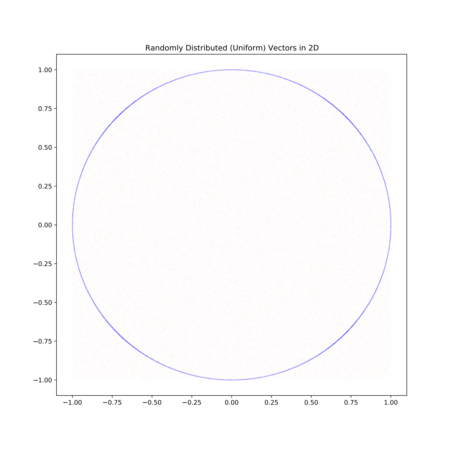
Do you notice the clumping?
Okay, maybe it’s not so obvious. I’ve made the dots somewhat transparent so that overlap would show up as darker regions. If you look at the four “diagonal” directions (North-West, North-East, South-West, and South-East), you will notice the blue is more prominent. That’s because there’s clumping in those regions. Those areas are denser than the regions at the regular cardinal directions (North, East, South, West).
Why does this happen?
To get a handle on this question, think about what we’re sampling when we use the uniform probability distribution. Any given coordinate is being chosen in an interval [-1,1], so in total our vector is being sampled from a box whose side length is 1−(−1)=2. For the plot above, this box is just a square, and you can see that the red dots do indeed sample the box at a pretty uniform rate (there’s no clumping that I can see).
When we sample uniformly from the coordinates, the space we sample is a box.
But what are we really trying to do when we want to sample unit vectors?
Not only do we want to pick the coordinates at random, we want the norm of the vector to be one. This modifies the geometry of our space. If the vector must have unit length, the space we want to sample should be spherical. Looking at any other space will introduce bias in our results.
Okay, let’s unpack this a bit.
A unit vector is a vector with length one. This means that if your vector has coordinates xi, then the coordinates satisfy:
∑i xi2 = 1.
If we’re in two dimensions, this is just a fancy way of writing out the Pythagorean theorem with hypotenuse of length 1. If you vary the coordinates of your two-dimensional unit vector, you will trace out a circle. In higher dimensions, we trace out spheres, which is why we call such an equation spherically symmetric.
This means that choosing a random unit vector with uniform probability requires us to sample from a spherically symmetric distribution. Or at the very least, if you don’t use a spherical geometry, whatever you do to rescale things should counter the bias you introduced. We’ll just focus on making our distribution symmetric to start with, and see why picking uniform Cartesian coordinates doesn’t work.
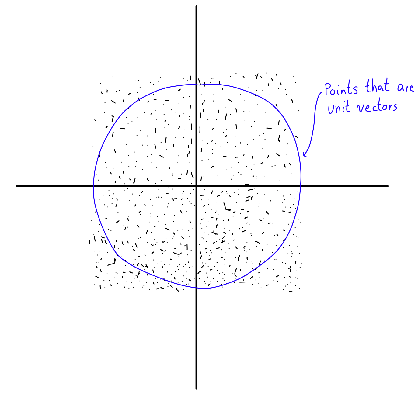
Sampling our Cartesian coordinates as indicated above gives us a square in two dimensions, which we can plot relative to the circle (the spherically symmetric unit vectors).
Imagine you generate a bunch of random points within the square. This is what generating uniformly random Cartesian coordinates gives us (with the blue circle being the points that are unit vectors):
Now, we want to modify those dots so they all become unit vectors. How do we do this? We rescale! Each vector has a certain distance from the origin, and it’s likely that this distance isn’t one, like so.
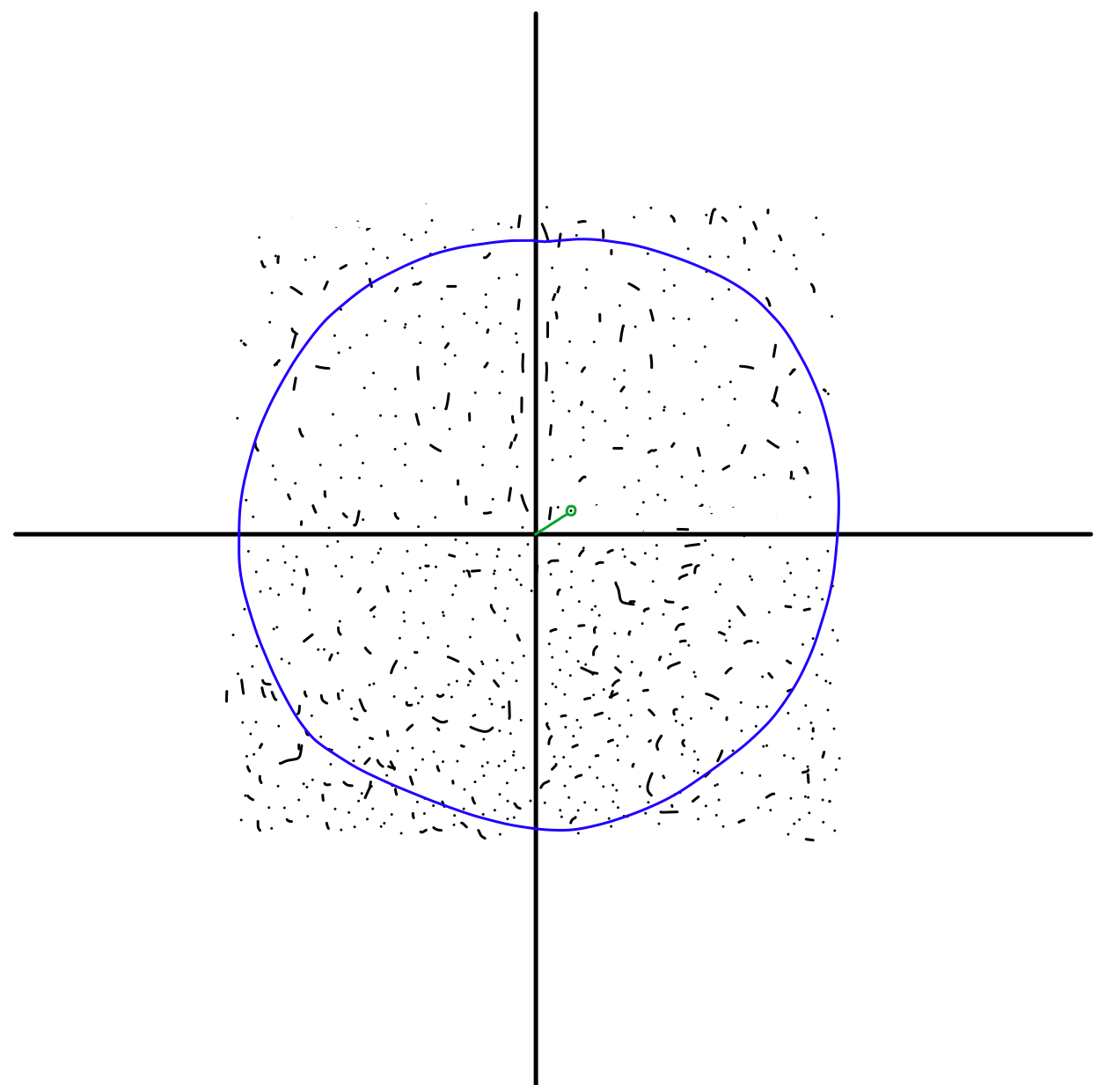
Using the coordinates of the point, we can calculate it’s length from the origin, then divide each coordinate by that length. Doing so will give you a unit vector by definition.
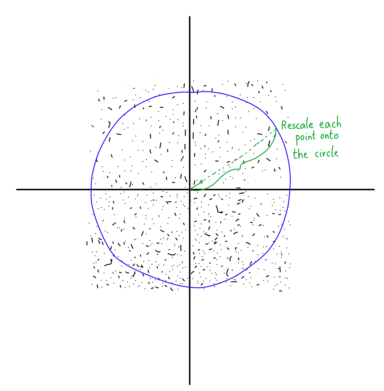
But what does this rescaling look like on our square of points?
We know that rescaling will either push a vector with length less than one or pull a vector with length greater than one onto the circle.
Here is the fun part. Look at the difference between the North-East and North directions. In the North, almost all the points are closer to the origin than the circle. In fact, if you’re looking exactly North, than the only points that aren’t closer to the origin are those that already lie on the circle at the point (0,1). Everything else is pushed upwards.
But look at what happens in the North-East. You still have the same amount of points that are closer to the origin than the circle (because the circle is spherically symmetric, this is true in any direction you look). However, now you have a ton of extra points that are further from the origin than the circle!
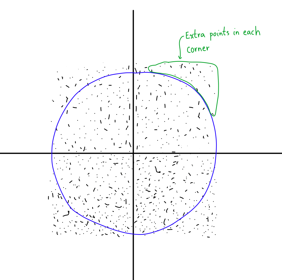
I like to think of these as “extra” points that get pulled in because of the geometry of the box. In essence, the box puts “more” points in the corners, so those get rescaled down and populated the diagonal directions with more points when we rescale.
This is exactly what I was referring to when I talked about “clumping”. Because there are a bunch of extra points in the corners, your sampling will end up producing more points in those directions than the regular cardinal directions.
Here’s another way to think about. If you look in the North direction, you can go at most 1 unit away before you hit the box. This means that you have one unit of “space” to generate points on that line. But in the diagonal directions, you now have √2 units for your points to land on! Since your line is longer, more points will accumulate on it, making those directions favoured (biased).
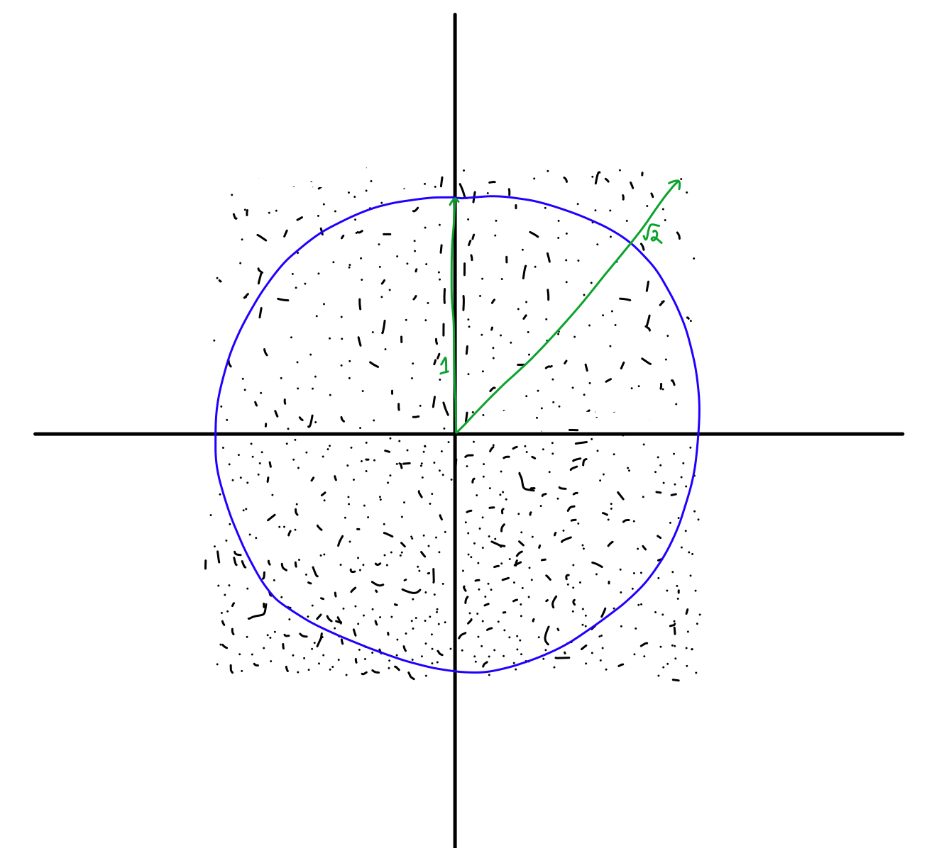
When you use Cartesian coordinates that are sampled uniformly, you end up generating many more “corner samples” than you would want.
And it gets worse. How much “extra space” is there in a box compared to a sphere? In two dimensions, the area of a unit circle is π, and the box has area 22 = 4, so the ratio is π/4≈0.785. This means that there’s about 21.5% “extra space” between them.
In three dimensions, the volume of a unit sphere is (4/3)π, and the box’s volume is 23 = 8, so the ratio is (4/3)π/8≈0.524. As we can see, we have a lot more extra space!
If we look at the ratio in n dimensions, we need to know the sphere’s volume. Using Stirling’s formula (an approximation for factorials), the volume of a unit n-sphere is:
Vs(n) ~ (1/nπ)1/2(2πe/n)n/2.
We won’t dive into the reasoning here (perhaps in another essay). The volume of the box is much simpler. Each size as a factor of 2, so the volume is 2n. Therefore, the ratio looks like:
Vs(n)/2n ~ (1/nπ)1/2(πe/2n)n/2 → 0 as n → ∞.
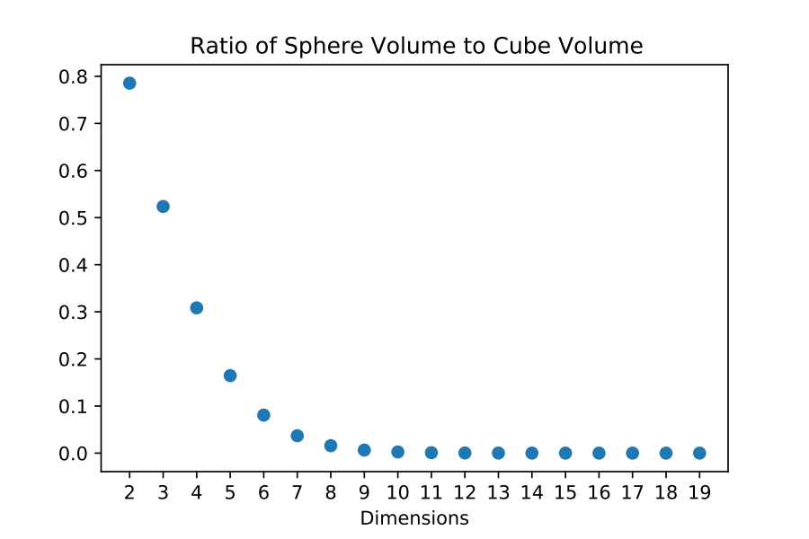
Put more colorfully: As you go to higher dimensions, your box becomes almost entirely filled in the corners. This means the bias we’ve seen in two dimensions will only get worse.
When you’re in high dimensions, everything is in the corners.
The normal way
So what’s a good way to generate these unit vectors then?
One answer lies in taking a detour to see a certain kind of distribution, called a Gaussian or normal distribution. This distribution is one you see all over probability theory. In fact, I’d wager that saying “probability theory” will generate thoughts of the normal distribution in the minds of mathematicians.
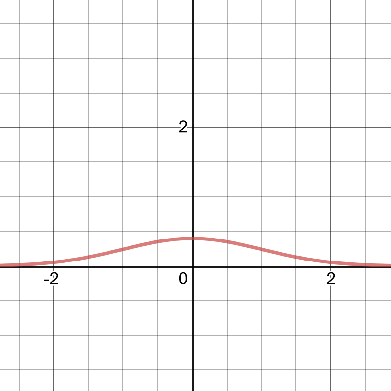
What is the normal distribution? Briefly, the idea is that most of the possible values the distribution can take will be centered at a mean μ, and the the probability of getting a value away from the mean tapers off (controlled by a parameter σ called the variance). Mathematically, it looks like:
\(f(x) = \frac{1}{\sigma \sqrt{2\pi}} \exp{\left[ -\frac{1}{2} \left( \frac{x-\mu}{\sigma}\right)^2 \right]}.\)
This may look like an intimidating function, but when you plot it, the reality is much simpler.
The wonderful thing about a function like the exponential is that it transforms multiplication into addition. This is one of the laws that get taught to secondary students early on:
eaeb=ea+b, where a and b are numbers.
This is going to be hugely helpful to us.
We’ve seen graphically that a uniform distribution doesn’t give us a spherically symmetric distribution. What makes this distribution different? After all, we’re still going to sample each Cartesian coordinate independently, so what’s the big deal with the normal?
It all has to do with the joint probability distribution.
Let’s go back to our two-dimensional case. Here, we have our x and y coordinates that we want to sample. We can don’t really care about rescaling after, but it needs to be done in a way that everything stays spherically symmetric.
The joint probability distribution simply tells us how to link together multiple probability distributions. Because we’re looking at independent coordinates, our joint probability distribution will satisfy:
\(f(x,y) = f(x)f(y).\)
In the uniform case, we have f(x) = f(y) = 1/2, where the 2 comes in because it’s the length of the interval. This nets us a “square” distribution for the coordinates, which doesn’t respect spherical symmetry.
On the other hand, if we take a normal distribution with mean zero (μ=0) and variance one (σ=0), the joint distribution will look like this:
\(f(x,y) = f(x)f(y) = \frac{1}{2\pi} \exp{\left[-\frac{1}{2} \left( x^2 + y^2 \right) \right]}.\)
Look at the argument of the exponential. Does the expression x2+y2 look familiar?
This is precisely the radius r in polar coordinates! If we make the substitution, we end up with:
\(f(x,y) = f(r).\)
This is the reason that sampling from a normal distribution works. The structure of the exponential transforms a multiplication from independent distributions to an addition in the exponential. Furthermore, the fact that we have the square of the variable lets us employ the trick of going to polar coordinates.
Now that our distribution is a function of r, we’re guaranteed for it to be spherically symmetric. This means we’ve successfully constructed a way to sample unit vectors! All we have to do is the following.
- For each Cartesian coordinate, sample a number from the probability distribution N(0,1) (the normal distribution with μ=0 and σ=1).
- Rescale the vector you generate by its magnitude.
And that’s it! By simply changing the distribution we sample from, we can encode the fact that we want a spherically symmetric distribution.
——
Probability is a subtle mathematical subject, with the answer you get often hinging on the assumptions you baked into your approach (which are often implicit!). We saw a small example here, but this shows up everywhere in mathematics, and what it teaches me is that we need to be careful when tackling a problem. It’s worth spelling out your assumptions, checking to see if there are unintended consequences, and mending them if necessary.
This essay showed up that asking a simple question (How can I generate random unit vectors?) can lead us astray if we don’t question our assumptions. The probability distribution we used on the first try “fills up the corners” of our hypercube, bringing with it unwanted clumpy-ness. It also showed us that high-dimensional objects have properties that might run against our initial guess.
So the next time you start looking at hyperspheres and hypercubes, remember: the volume goes all to the corners.
References
- For more on the n-sphere and its geometrical properties, see this Wikipedia article. There are plenty of interesting nuggets in higher dimensions, and many of them are collected here.
- This StackOverflow question is how I got started when I wanted to implement this in Python.