Hilbert space is big.
No, not big like the how the Earth is big compared to you. Rather, Hilbert space is astronomically big. Actually, that’s not quite right either. It’s bigger than that. I guess the best adverb I can use is that it’s mathematically big. In a Hilbert space, you tend to have a lot of room to maneuver. (To read more about that, check out my essay, “The Curse of Dimensionality”.)
In the last essay, we saw how to pick a random unit vector in a N dimensional space. This wasn’t for nothing, and now we are going to put that knowledge to use to ask the following question:
If I have a line of N qubits and randomly pick a state from the Hilbert space, what kind of entanglement will it have?
The essence of this question revolves around the idea of trying to capture what a quantum state is like. The reason we care is because some quantum states are much easier to engineer than others. For example, if we have the state $|0\rangle |0\rangle$, it’s much easier to prepare than the state $\frac{1}{2} \left(|0\rangle|0\rangle + |1\rangle|1\rangle \right)$. This is because the latter state is entangled, and generating purposeful entanglement can be tricky.
Plus, simulating quantum systems accurately means you have to track the exponential number of states it can be in, and entanglement is partly the reason why you can’t only consider a few of those exponentially many states. As such, it’s worth thinking about what the average case looks like.
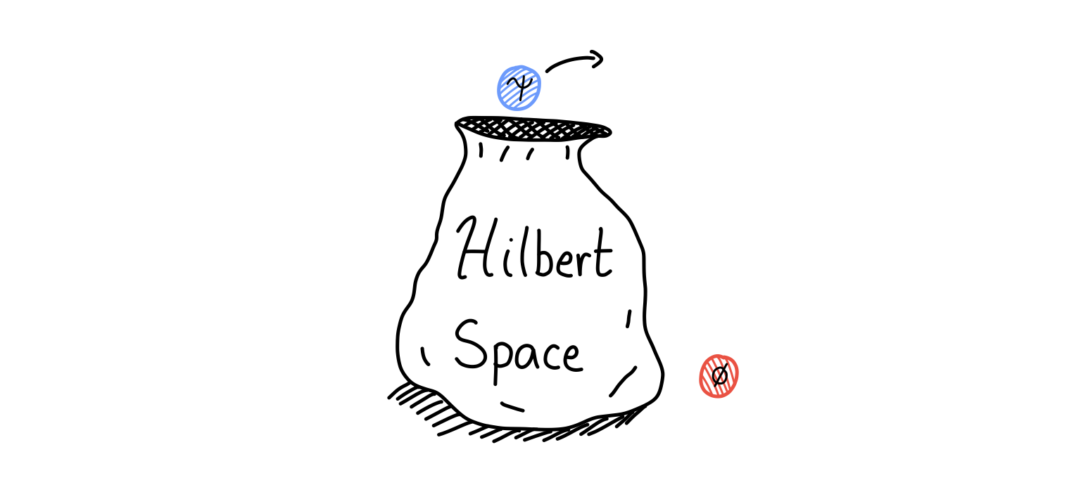
Not only that, but this is the kind of question a physicist likes to ask. We don’t tend to study quantum states but quantum systems, which effectively means we are studying at the Hilbert space level. For the purposes of this essay, think of Hilbert space as a bag which contains a bunch of balls, each one a quantum state. Than, our question from before becomes: If I pick a ball from the Hilbert space bag, how much entanglement can I expect it to have?
This question will make us cover a lot of ground. We’ll see what to use as a measure of entanglement, we will talk about one of the most useful tools in linear algebra that quantum physicists use all the time, and we will (naturally) make a few approximations to help smooth our way. It promises to be a fun ride, filled with plenty of fun mathematical morsels to ponder.
Let’s go!
A Quantum Cut
If we want to quantify entanglement, we need to first talk about how to partition quantum states. In particular, we’re going to look at the simplest partitioning scheme: cutting a quantum state into two parts (called a bipartition).
The idea is straightforward. Imagine we have a quantum state over four qubits:
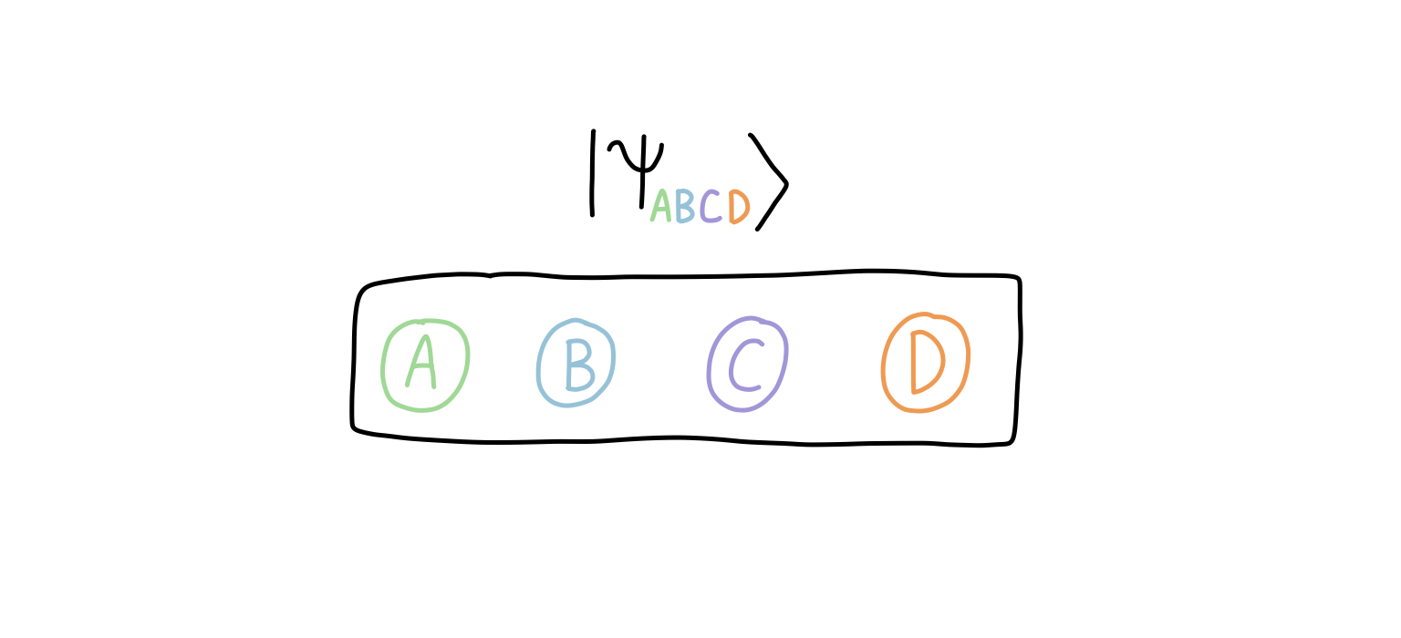
Then, a bipartition of the quantum state corresponds to inserting a “cut” so that the qubits are separated into two groups (I’ve shown multiple ways here):
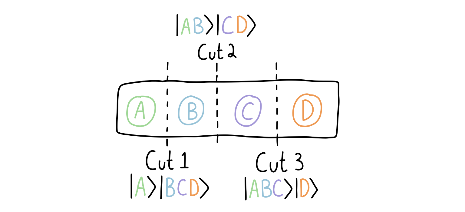
Do we have to cut the states in the middle? No! But in our case, we will because it seems the conceptually easiest to do when we’re talking about average cases. But in principle you could cut the state anywhere you want, and this would give you a different bipartition of the system into parts A and B. You could even go crazy and group qubits that aren’t adjacent, though that’s beyond what we will do.
How does this get reflected in the mathematics?
Let’s start with a our quantum state over four qubits. Then, if I write the state of each qubit in the computational basis, the whole state can be written as:
\(|\psi\rangle = \sum_{i,j,k,l} c_{ijkl} |i\rangle |j\rangle |k\rangle |l\rangle.\)
The tensor $c_{ijkl}$ holds all of the coefficients we need for the quantum system. If you’re not used to this notation, it just means that there’s a coefficient for every combination of $i,j,k,l$. But the problem is that, written this way, we can’t cut things in a clean way such that the $i$ and $j$ part become one factor, and the $k$ and $l$ part become another. We would need more information about the quantum state to do this. In other words, we can’t perform the following “factoring” of the sums:
\(\sum_{i,j,k,l} c_{ijkl} \nrightarrow \sum_{i,j} a_{ij} \sum_{k,l} b_{kl}.\)
For example, if we had the state $|\psi\rangle = |0\rangle |1\rangle |1\rangle |0\rangle$, then the only nonzero coefficient would be $c_{0110} = 1$, so we could then actually break up the system into $|\psi\rangle = |A\rangle |B\rangle$, where $|A\rangle = |0\rangle |1\rangle$ (over the first two qubits) and $|B\rangle = |1\rangle |0\rangle$ (over the final two qubits).
The point here is that we can cut our system into two parts, A and B, and there’s only one term. Notice that I did not write a sum for the state in terms of A and B. That’s key, and it’s what will let us define entanglement.
But let’s back up. If we have the state given by the coefficient tensor $c_{ijkl}$, then can we still write the sum in terms of a system A and a system B?
The answer is yes! The price we pay though is that we might not get only one term for our result.
The tool we need to cut our system into two parts is called the Schmidt decomposition. This is the tool I go back to again and again in my research, because it forms the bedrock of how I classify quantum states. We won’t prove the Schmidt decomposition in the essay (perhaps another one in the future), but instead I’ll give you the idea. If you want to know more, I highly recommend looking at Tai-Danae Bradley’s work in Reference 1.
The Schmidt decomposition gives us a way to “split” a quantum system into two parts, in such a way that the coefficients only depend on a shared index. If we’re dealing with a bipartite system (two parts), then this means the coefficient matrix is diagonal.
Take a state on two qubits, which we can write as:
\(|\psi\rangle = \sum_{i,j} c_{ij} |i\rangle |j\rangle.\)
Notice that the coefficients depend on both $i$ and $j$. Moreover, the whole state involves two sums. What the Schmidt decomposition will do is reduce our state to something that looks like this:
\(|\psi\rangle = \sum_{a} c_{aa} |a\rangle_1 |a\rangle_2.\)
Now, the sum has only one index to go over ($a$), and the coefficient matrix is diagonal.
Why is this useful? It has to do with the fact that we can quantify entanglement with these values. They are the eigenvalues of our system, and are also called the Schmidt values.
In fact, the idea of calling a quantum state entangled rests precisely on this summation over $a$. If the index only takes one value, then we say the state is not entangled. However, if the index takes more than one value, the state is then entangled.
We often don’t write something like $c_{aa}$. Instead, we just give it one index, so it would like something like $c_a$. This emphasizes that it’s not an index of either system in particular, but in fact something that characterizes both.
In terms of performing the Schmidt decomposition, the proof is actually constructive. We follow an algorithm that amounts to finding the eigenvalues of the system (with a singular value decomposition of the form $udv$, which you can also look at Reference 1 to learn about), and then rotating the quantum state basis vectors with the matrices $u$ and $v$, while the matrix $d$ (a diagonal matrix) holds the Schmidt values.
Once we decompose our system like this, we now have an easy way to calculate the amount of entanglement in the state.
Quantifying entanglement
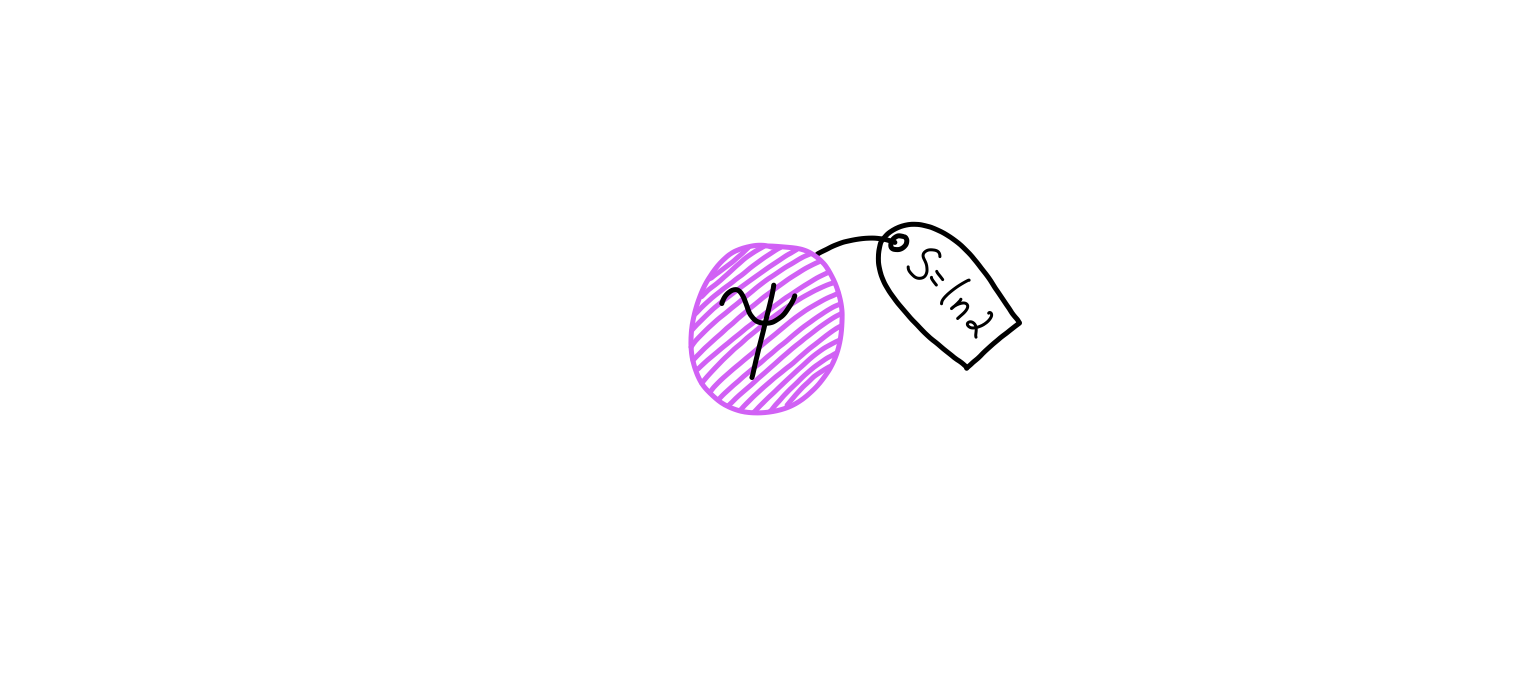
Before we even start solving our problem, it’s worth thinking about what I mean when I say “the entanglement of a quantum state”. After all, quantum states don’t come with little price tags that announce how much entanglement they have! Rather, we need to come up with a notion for how entangled a quantum state is.
There’s a lot of literature on this question (and a bunch of associated measures), but we will just look at one of the simplest ones: the Schmidt values.
As we saw above, if we have a quantum system we can partition it into two systems, perform the Schmidt decomposition, and end up with something that looks like (where we split the system into parts A and B):
\(|\psi\rangle_{AB} = \sum_{a} \lambda_{a} |a\rangle_A |a\rangle_B.\)
One of the reasons we like this decomposition is that it gives us a way to easily calculate what’s called the “entanglement entropy” (or “entropy of entanglement”). It’s a measure that works for a pure state, which is what we have above. If we then consider the density matrix given by $\rho_{AB} = |\psi\rangle \langle \psi|$, This quantity is calculated using the following equation:
\(S(\rho_A) = -\text{Tr}\left( \rho_A \ln \rho_A \right).\)
Here, $\rho_A$ is the density matrix you get from doing an operation called “tracing out” system B. This gives us an idea of the state only on A, and if there was any entanglement in the original AB system, it will show up here.
You might be thinking that it’s awfully weird to calculate the entanglement entropy of $|\psi\rangle_{AB}$ using only half of the system, but the above definition is actually symmetric. In other words, $S(\rho_A) = S(\rho_B)$. In fact, because we have our state in the Schmidt decomposed form, we can do a bit of algebraic magic to eventually end up with:
\(S(\rho_A) = - \sum_a \lambda_a^2 \ln(\lambda_a^2).\)
In a future essay, we’re going to look at a different kind of entanglement that can arise. In this case, the quantum state’s entanglement entropy isn’t related to its volume, but its area. This is usually called the “area law”, but as we will see later on, it’s probably better to call it a “boundary law”. In either case, this will let us study systems whose growth of entanglement doesn’t grow with system size, giving us hope for studying these systems in more depth.
But that’s for another essay! For us, we will see that picking a random quantum state gives us entanglement that grows with the system size.
Volume law
When we look at the entanglement entropy of one of these random quantum state (on two different Hilbert spaces of size $m$ and $n$, with $m\leq n$, the average entropy scales as:
\(\langle S(\rho_A) \rangle \approx \ln m - \frac{m}{2n}.\)
I’ve included some references at the end that go into this result (see References 2 and 3). To show the full-blown calculation will take us way outside what I want us to explore today. Instead, I want to give you a taste for why an expression like this makes sense. To do that, we’ll play the usual game of a physicist who wants to show something without a care for total rigour: handwaving and appeals to idealizations. Don’t worry though, the steps will be instructive.
If we start by writing out our random quantum state, it will look like what we had before:
\(|\psi\rangle = \sum_{i}^m \sum_{j}^n c_{ij} |i\rangle |j\rangle.\)
Since we’re picking random unit vectors, we know from “All in the Corners” that we want to sample from a unit hypersphere. As a probability distribution, this means we want our coefficients to follow (where c is all of our coefficients):
\(P(c) \sim \delta \left( \sum_i^m \sum_j^n \lvert c_{ij} \rvert^2 - 1 \right).\)
Okay, this might not be the most transparent of expressions, so let’s walk through what it means.
The term inside of the parentheses measures the difference between the sum of the squares of the coefficients from 1. Remember that this double sum is just computing the “radius” of the vector c which describes our coefficients. This is exactly what we looked at in the previous essay, where we wanted the sums of squares to be equal to 1. So the expression in the parentheses is measuring how close we are to 1.
Then, the $\delta$ is the symbol used for the Dirac delta distribution. Sweeping a bunch of details under the rug, the Dirac delta distribution is 1 if the argument in the parentheses is 0, and is zero everywhere else. This effectively means we “pick out” the vector c such that our coefficients are normalized to one. Everything else is not allowed.
Finally, we don’t have a strict equality because there may be a normalization factor. However, we won’t worry about it because we will switch to a different distribution soon.
While compact, this expression is only nice to work with under certain circumstances. This isn’t one of those times.
Remember, the end goal is to estimate the average entanglement entropy of our two-system state, $\langle S(\rho_A) \rangle$. This means we need a probability distribution for the states to follow, and this is what our Dirac delta distribution above is for us.
If we use the expression for the entanglement entropy I wrote above, the average is computed as:
\(\langle S(\rho_A) \rangle
= - \left\langle \sum_i^m \lambda_i^2 \ln \lambda_i^2 \right\rangle.\)
This expression is fine, but it hides something tricky. The angular brackets mean we have to take the expression within and evaluate it against a probability distribution. In terms of notation, we have:
\(\left\langle \cdot \right\rangle \equiv \int \left( \cdot \right)P dP.\)
Here, $P$ is our probability distribution. Also, while I’ve written an integral for our expression here, that’s not the only possibility. It could be a sum if we’re dealing with discrete objects. Since the possible coefficients are continuous though, the integral is appropriate.
So what is our probability distribution? It looks like we could just use our equation for $P(c)$, but the problem is that our entropy is expressed in terms of the Schmidt values $\lambda_i$, while our probability distribution is expressed in terms of $c_{ij}$. We will have to deal with this in some manner, but let’s leave it be for now.
We can start by writing the Schmidt values as:
\(\lambda_i^2 = \frac{1}{m} + \delta_i, \,\,\, \delta_i \in \mathbb{R}.\)
This might not look really useful, but there are two things to note here. First, this decomposition is of the form “constant” + “fluctuation”. In fact, the constant part $1/m$ is simply the contribution we would get if the state was uniform (which means maximum entropy). The upshot is that in our expression for the logarithm, we will be able to expand things to get a constant part and a fluctuating part.
Second, because our quantum state needs to be normalized, we have the following implication:
\(\sum_i^m \lambda_i^2 = 1 \rightarrow \sum_i^m\frac{1}{m} + \sum_i^m \delta_i = 1 \rightarrow \sum_i^m \delta_i = 0.\)
This will help us out later, so let’s keep it in our back pocket.
We’re now in a position to expand the logarithm using a Taylor series, which gives us:
\(\ln\left( \frac{1}{m} + \delta_i \right) = - \ln m + \sum_{k=1}^\infty \frac{(-1)^{k-1}}{k} (m\delta_i)^k.\)
This looks complicated, but it will allow us to take in each piece of the problem separately. If we write out what the integral looks like, it will be (following the notation of Reference 3):
\(\langle S(\rho_A) \rangle = \ln m - \frac{m}{2} \left\langle \sum_i \delta_i^2 \right\rangle + \frac{m^2}{6} \left\langle \sum_i \delta_i^3 \right\rangle - \ldots\)
Where did all of these terms come from? They all come from this big multiplication:
\(\langle S(\rho_A) \rangle = - \left\langle \sum_i^m \left( \frac{1}{m} + \delta_i \right) \left( - \ln m + \sum_{k=1}^\infty \frac{(-1)^{k-1}}{k} (m\delta_i)^k \right) \right\rangle.\)
If we multiply the first two terms of each expression, we see that we get:
\(-\left\langle \sum_i^m \left( \frac{1}{m} \right) \left( - \ln m \right) \right\rangle = \frac{\ln m}{m} \sum_i^m 1 = \ln m.\)
The other terms follow this exact method, though you need to keep the angular brackets because the terms with $\delta_i$ do depend on the various values of $\lambda_i$.
For our purposes, we will only look at the first two terms (there should be an argument about the higher terms being negligible when $n$ becomes large). That means our last step is to evaluate the $\delta_i^2$ term.
We will go about this in an oblique way. Remember that this term is related to the eigenvalues $\lambda_i$. But the probability distribution for them is not available to us (at least, without a lot of work), but we do have the probability of picking our coefficients $P(c)$.
To get there, we will first notice that we can calculate the trace of our density matrix pretty easily when we have the Schmidt decomposed form (the one with $\lambda_i$).
Because the matrix is diagonal, the trace is just the sum of those components. If we take the trace of a density matrix, it’s always one (that’s the normalization). It’s also why the average of the sum of $\delta_i$ is zero. But unless we’re dealing with a pure state, the trace of $\rho^2$ isn’t one. In fact, this quantity is called the purity of a state because it’s one if and only if the state is pure.
The good news is that we can still compute the trace easily:
\(\text{Tr}\rho_A^2 \equiv \sum_i^m \lambda_i^4 = \sum_i^m \left( \delta_i + \frac{1}{m} \right)^2 \\
= \sum_i^m \delta_i^2 + \frac{2}{m}\sum_i^m \delta_i + \sum_i^m\frac{1}{m^2} = \sum_i^m \delta_i^2 + \frac{1}{m}.\)
The point is that we can now substitute our average over $\delta_i^2$ for an average over the trace of our reduced state, which we will be able to calculate. In other words:
\(\left\langle \sum_i^m \delta_i^2 \right\rangle = \left\langle \text{Tr}\rho_A^2 - \frac{1}{m} \right\rangle.\)
Putting everything together, our average entropy looks like:
\(\left\langle S(\rho_A) \right\rangle = \ln m - \frac{m}{2} \left\langle \text{Tr}\rho_A^2 - \frac{1}{m} \right\rangle.\)
So we’ve kicked our problem down the road. We’re almost at an expression for the entropy, but we have this pesky trace over the square of the density matrix. This isn’t exactly forthcoming with insight, so we’d like to deal with this term.
Relaxing the Delta
To do this, we will now make use of our probability distribution from the beginning. Remember that it looks like this:
\(P(c) \sim \delta \left( \sum_i^m \sum_j^n \lvert c_{ij} \rvert^2 - 1 \right).\)
But dealing with a Dirac delta distribution isn’t fun unless you’re in very specific scenarios. Therefore, we will relax this distribution to one which is much easier to do calculations. We will end up getting the same asymptotic result at the end, and save ourselves some algebra.
Instead of sampling from this distribution, we’re going to use a modified distribution that will approximation $P(c)$. I’ll give it the name $Q(c)$, and it will look like:
\(Q(c) = \prod_{i,j} \frac{nm}{\pi} \exp{\left( -nm |c_{ij}|^2 \right)}.\)
Those sharp-eyed readers will recognize this as nothing other than a product of Gaussian distributions for the coefficients $c_{ij}$ with the mean being zero ($\langle c_{ij}\rangle = 0$) and variance $\langle |c_{ij}|^2\rangle = 1 /nm $.
Why does this distribution make sense?
First, the mean being zero just tells us that we aren’t biasing the distribution towards one direction or another. Second, the variance being $1/nm$ encodes the fact that we want the state to be normalized. Remember that the trace of the density matrix has to be one. But with this Gaussian distribution, it’s not quite equal to one, since we aren’t using the Dirac delta.
Those in physics are used to this substitution though. A Dirac delta distribution can be approximated using a Gaussian distribution, and this is exactly what we are doing here. Graphically, you can see this in the following animation that starts with a Gaussian distribution and sends $nm\rightarrow \infty$.
From the animation above, you see that the peak gets more sharply defined and narrower as time goes on. This shows us that our Gaussian function can approximate a Dirac delta distribution better and better.
We can now compute some of the traces we need. First though, we calculate the reduced density matrix $\rho_A$, which is defined as $\text{Tr}_B \rho_{AB}$.
\(\rho_{AB} = |\psi\rangle \langle\psi| = \sum_{i}^m \sum_{j}^n c_{ij} |i\rangle |j\rangle \sum_{k}^m \sum_{l}^n c^*_{kl} \langle k| \langle l| \\
= \sum_{i,k}^m \sum_{j,l}^n c_{ij} c^*_{kl} |i\rangle\langle k| \otimes |j\rangle \langle l|.\)
A bit of a monster expression, but the terms are grouped up for us to easily take the partial trace over subsystem B.
\(\rho_A =\sum_{i,k}^m \sum_{j,l}^n c_{ij} c^*_{kl} |i\rangle\langle k| \text{Tr} \left( |j\rangle \langle l| \right) = \sum_{i,k}^m \sum_{j,l}^n c_{ij} c^*_{kl} |i\rangle\langle k| \delta_{jl} \\
= \sum_{i,k}^m \sum_j^n c_{ij} c^*_{kj} |i\rangle\langle k|\)
Then, we can look at the trace of $\rho_A$, which we know should be one if we’re following our Dirac distribution, but might be off a bit here.
\(\text{Tr}\rho_A = \sum_{i,k}^m \sum_j^n c_{ij} c^*_{kj} \text{Tr}\left(|i\rangle\langle k| \right) = \sum_{i,k}^m \sum_j^n c_{ij} c^*_{kj} \delta_{ik} \\
= \sum_{i}^m \sum_j^n |c_{ij}|^2.\)
The problem is that the Gaussian distribution doesn’t have this being equal to one. But, on average this will be true, because of the requirements we set on the coefficients from before:
\(\left\langle \text{Tr}\rho_A \right\rangle = \left\langle \sum_{i,j}|c_{ij}|^2 \right\rangle = \sum_{i,j} \left\langle|c_{ij}|^2 \right\rangle = \sum_{i,j} \frac{1}{mn} = 1.\)
This means that on average, our state is normalized (which we are certainly hoping for!).
We now need to deal with the other term, which involves $\rho_A^2$. So first, we take a deep breath, dig into the algebra, and calculate it:
\(\rho_A^2 = \sum_{i,k}^m \sum_j^n c_{ij} c^*_{kj} |i\rangle\langle k| \sum_{a,d}^m \sum_b^n c_{ab} c^*_{db} |a\rangle\langle d| \\
= \sum_{i,k, a,d}^m \sum_{j,b}^n c_{ij} c^*_{kj} c_{ab} c^*_{db} |i\rangle\langle k| a\rangle\langle d| \\
= \sum_{i,k, a,d}^m \sum_{j,b}^n c_{ij} c^*_{kj} c_{ab} c^*_{db} \delta_{ka} |i\rangle\langle d| \\
= \sum_{i, a,d}^m \sum_{j,b}^n c_{ij} c^*_{aj} c_{ab} c^*_{db} |i\rangle\langle d|.\)
Yes, there are a lot of indices to keep track of! Now, we’re in a position to trace over this to find the purity.
\(\text{Tr}\rho_A^2 = \sum_{i, a,d}^m \sum_{j,b}^n c_{ij} c^*_{aj} c_{ab} c^*_{db} \text{Tr} \left(|i\rangle\langle d|\right) \\
= \sum_{i, a,d}^m \sum_{j,b}^n c_{ij} c^*_{aj} c_{ab} c^*_{db} \delta_{id} \\
= \sum_{i, a}^m \sum_{j,b}^n c_{ij} c^*_{ib} c_{ab} c^*_{aj}.\)
Okay, still not the most comprehensible. What we’re going to do though is exploit the properties that we were choosing our states with. Namely, that the coefficients have mean zero and variance $1/nm$.
How does this help?
Let’s split our sums into parts. If you look at the coefficients $c_{ij}c^*_{ib}$, they are just begging to have $j = b$ so we can combine them. That’s going to be our strategy here. In fact, we’re going to do a decomposition of the form:
\(\sum_{i, a}^m \sum_{j,b}^n = \sum_{i, a}^m \sum_{j=b}^n + \left( \sum_{i = a}^m \sum_{j\neq b}^n + \sum_{i\neq a}^m \sum_{j \neq b}^n \right).\)
This covers all of the different possibilities for the sum. The first term is when $j = b$, and the second term in parentheses is when $j\neq b$ (just split up even further). We can then use our properties from the sampling.
Let’s look at the first term. Since $j = b$, we will have:
\(\sum_{i, a}^m \sum_{j=b}^n |c_{ij}|^2 |c_{aj}|^2.\)
By itself, not that interesting. But if we look at the average (which is our goal), we get:
\(\sum_{i, a}^m \sum_{j=b}^n \left\langle|c_{ij}|^2 \right\rangle \left\langle|c_{aj}|^2\right\rangle = \sum_{i, a}^m \sum_{j=b}^n \frac{1}{\left(mn\right)^2} = \frac{m^2n}{m^2n^2} = \frac{1}{n}.\)
The reason we can just take the product of the averages has to do (I think) with the fact that the coefficients are sampled independently, so there shouldn’t be an “cross-talk” between them.
The next piece is when $i=a$ and $j\neq b$. This gives us another nice grouping of the coefficients:
\(\sum_{i = a}^m \sum_{j\neq b}^n |c_{ij}|^2 |c_{ib}|^2.\)
It’s a similar story to the previous one when we take the average. The only difference is that now $j\neq b$, so there are slightly less terms in the sum:
\(\sum_{i=a}^m \sum_{j \neq b}^n \left\langle|c_{ij}|^2 \right\rangle \left\langle|c_{ib}|^2\right\rangle = \sum_{i= a}^m \sum_{j\neq b}^n \frac{1}{\left(mn\right)^2} = \frac{mn(n-1)}{m^2n^2} \\
\approx \frac{1}{m} \,\,\, \text{for} \,\,\, n \rightarrow\infty.\)
The last term is the easiest. Here, we have $i\neq a$ and $j \neq b$, which means that none of the coefficients will group up. Instead, when we take the average, we will be able to invoke the property of our coefficients having mean zero, so this term won’t contribute.
All told, our end result (in the asymptotic limit of large $n$) is this:
\(\left\langle \text{Tr}\rho_A^2 \right\rangle \approx \frac{1}{n} + \frac{1}{m} = \frac{m+n}{mn}.\)
How does this compare with the exact expression? It turns out that the only difference (see Reference 3) is that the denominator becomes $mn+1$, which we know won’t make a ton of difference when the size of our Hilbert spaces are very big.
So, going all the way back to our calculation for the average entropy, we find that we get:
\(\left\langle S(\rho_A) \right\rangle \approx \ln m - \frac{m}{2} \left\langle \text{Tr}\rho_A^2 - \frac{1}{m} \right\rangle \\
\approx \ln m - \frac{m}{2} \left( \frac{1}{m} + \frac{1}{n} - \frac{1}{m} \right) \\
= \ln m - \frac{m}{2n}.\)
I don’t know about you, but isn’t it nice we could get to a simple result in the end without too many simplifications?
This result is sometimes called the Page limit, and it shows us that the average entropy of a quantum state in a Hilbert space is almost maximal. The maximal part is from the $\ln m$, which is what you get when you do an analysis for the maximum entropy a system can have (basically, when the probability distribution for your states is uniform).
But why is this important?
Remember that $m$ and $n$ are the dimensions of our Hilbert spaces. So if we have $A$ qubits in the first system and $B$ qubits in the second system, then $m = 2^A$ and $n = 2^B$. If we imagine our system has the same number of qubits in both systems (so $A=B$), then our average entropy becomes:
\(\left\langle S(\rho_A) \right\rangle \approx \ln 2^A - \frac{1}{2} \\
= A\ln 2 - \frac{1}{2}.\)
What this means is that the entropy scales with the size of the system. Because we are in one dimension (just a line of qubits), you might even say the entropy is scaling with the volume. This is why physicists sometimes refer to a “volume law of entanglement”. They are talking about precisely this notion. When the entanglement entropy of the system scales with the system size, we call it a volume law.
So if I reach into my Hilbert space bag and pull a state out at random, not only will it be entangled, but it will be nearly maximally entangled.
The thing is, a lot of the states we’re used to seeing in physics are not maximally entangled. In other words, they don’t follow a volume law. These include product states that we use to start off computations in a quantum computer and the ground states of many Hamiltonians. So what’s the deal with them?
This leads to both a hypothesis, and a different type of entropy law. Whereas this essay showed you that grabbing a random state out of Hilbert space will net you one that follows a volume law, it turns out that a lot of states that are relevant for us physicists do not follow a volume law. In fact, many follow an area law, and this lack of growth in the entropy gives us hope that we can simulate a lot of these systems without even needing to use powerful quantum computers.
But that’s for a future essay. Here, just remember that you might not know the specific price tag of a particular quantum state, but you can be fairly sure that if you pick randomly, it will scale with the size of the system.
References
- “Understanding Entanglement With SVD”, Tai-Danae Bradley’s post on Math3ma for the Schmidt decomposition and looking at quantum states. She also does other interesting work on the crossroads of tensors, categories, and quantum theory. It’s worth reading the posts just for the lovely diagrams!
- “Average Entropy of a Subsystem”, by Don Page. This paper gives the result (Equation 10 of the paper) we get in this essay, with some additional corrections. I haven’t read through this super carefully, but it’s a derivation from the physicist’s perspective.
- “Many-body physics from a quantum information perspective”, by Remigiusz Augusiak, Fernando Cucchietti, and Maciej Lewenstein. This paper is the basis for this post, and it includes the suggestion of using Gaussian functions instead of discontinuous Dirac deltas for the probability distribution of being on a unit hypersphere. The relevant part is section 3.1.
I haven’t gone into this much, but it seems like the authors cite Lubkin’s paper which goes into more of the mathematical details, if you’re so inclined (warning: I didn’t read this paper myself and it might be behind a paywall).
Endnotes