If there’s one field of mathematics that everyone encounters in their daily life, I would argue that it’s combinatorics (with perhaps geometry being the other one). The rules of combinatorics cast a shadow over our lives. They affect how we make decisions and form the scaffolding for how options in our lives are displayed to us.
In this essay, I want to explore the idea which is known as the curse of dimensionality. It’s a lovely name, and the core of the concept is something that comes up without even straying too far into physics or mathematics (but we’ll get there!). To illustrate this, let me paint a little story.
Imagine you decide to start running. Of course, you need to purchase some running shoes, so you go to the store to look at the options. At first, you don’t know anything about running shoes. They look more or less the same, and you judge them based on their looks. However, after talking with one of the salespeople, you learn that there are different kinds of running shoes. In particular, road running shoes and trail running shoes form two broad categories. However, there are then options within those two categories, such as racing/training shoes, minimalist/maximalist, zero drop or non-zero drop, weight, price, and so much more. Soon, you realize that if you want to explore all of those different options, there will be a lot of shopping to do.
Let’s see how the combinatorics work. If there are just road/trail shoes, then there are two options. However, if you then add in the sub-category of racing/training, we get 2×2 = 4 options. If we add in the other options (zero/non-zero drop and minimalist/maximalist) and split up weight and price into five sectors each, we find that there are now 2×2×2×2×5×5 = 400 options. That’s for only six categories! If you had no inkling of which shoe would be best for you, paying for 400 different configurations of running shoes would be a difficult sell, even for the most passionate runner.
How did we get so many options? It comes from the fact that each new option you add introduces a multiplicative effect to the total number of configurations. This is known as the “multiplication rule” in combinatorics, and it illustrates the curse of dimensionality. As soon as you start adding in a lot of combinations, the number of possible configurations skyrockets.
Here, the idea of “dimension” isn’t just a reference to spatial lengths. When mathematicians and physicists use the word “dimension”, we tend to be thinking about something slightly different. Putting aside the discussion of fractals and non-integer dimensions, the idea of a dimension is simply a coordinate you need to describe the state of your system. In the example of the running shoes, at first we only needed one coordinate: road or trail. This choice specified the shoe for us. Each time we added a new category, this became an extra dimension to consider. By the end, we had six categories, so the problem of choosing a good running shoe became a six-dimensional problem.
This may seem disconcerting, since we’re used to having two or three dimensions when we think of space. However, the “space” that the story refers to can be thought of as the state space of possible running shoes. The first four dimensions have two possibilities each (corresponding to the twos in the product above), while the last two dimensions have five possibilities each.
Okay, but we might not need to explore all 400 options to get an idea of what kind of shoe you like. Perhaps if we choose a few good points, we can get an overall feel for which shoes are better.
That’s a good idea, and it’s what we try to do all the time when searching through higher-dimensional space in physics and mathematics. The curse of dimensionality reflects the fact that these spaces are just too damn big to go wading through all the options. Instead, we need to be clever about how we’re going to learn something about the space without wasting more time than necessary exploring it.
For the rest of this essay, I want to highlight a few areas within physics, machine learning, and statistics where the curse of dimensionality sneaks into the foreground.
Quantum systems and the vastness of Hilbert space
An example in physics where this problem pops up all the time is in quantum systems, particularly many-body systems.
In A Game of Loops, we explored the surface code, a quantum system that can help us do quantum error correction. There, we saw that the complete quantum state is described by an N×N lattice that has a qubit at each site. Because of this, there are N2 physical qubits needed for the system.
How big is the state space of this system? Well, we first have to figure out how many degrees of freedom a single qubit has. Remember that we can write the quantum state of a qubit in the following way: ψ = (a,b), where a and b are just complex numbers whose magnitudes sum to one. This could make it seem like a qubit has four degrees of freedom (since a complex number has two degrees of freedom and there are two here), but the normalization constraint will eliminate one of them. Furthermore, it turns out that we can eliminate a second degree of freedom, which comes from the fact that the overall phase of a quantum state doesn’t play a role in the physics. Taking both of these into account, the total number of degrees of freedom in a qubit is two.
That seems rather harmless, but as we’ll soon see, this leads to devastating consequences when trying to tackle quantum many-body problems.
Back to our surface code. We have N2 physical qubits, and each one has (independently) two degrees of freedom. How many do we then have in total? Well, this is simply the multiplication rule in action (you can think of specifying the quantum state as a series of choices for each physical qubit). This means in total we will have 2N2 total states.
If there’s one thing you should be worried about when you see exponents, it’s a tower of exponents.
To get an idea of how this grows, look at the following table:
| N |
2N2 |
| 1 |
2 |
| 2 |
16 |
| 3 |
512 |
| 4 |
65536 |
| 5 |
33554432 |
| 6 |
≈ 6.87×10¹⁰ |
| 7 |
≈ 5.63×10¹⁴ |
As you can see, this is really some explosive growth. Things start off fine, grow rather quickly, and are even manageable at N = 5. However, as soon as increase the lattice by one more unit length, the state space becomes enormous.
No wonder my machine learning project during PSI struggled when dealing with larger lattices.
And remember, this is only for N < 10. We aren’t exactly in the huge numbers territory in terms of lattice sizes, but the state space has its own scaling behaviour that makes things very difficult. This is only exacerbated for quantum many-body systems, which can have huge values of N. That’s why a lot of these problems are intractable at the moment, since we simply do not have the computational resources to get to lattices of that size.
This brings us to machine learning. If you know anything about machine learning, it’s probably that this approach loves trudging through data (sometimes called “big data”). While this is true, there are also limits to what we can do. As the number of dimensions (degrees of freedom) grows, the amount of work it takes to search through the possible options becomes worse than finding a needle in a haystack.
Neural networks and hyperparameter tuning
For my PSI project, the goal was to create an RNN decoder for the surface code (I will write about this more in a later essay). While the specifics aren’t super important, the key point is that neural networks aren’t magical. They take work to get right, and there are way more things you have to manually fiddle with than what you might expect.
Before I got into machine learning, I had the impression that building neural networks involved coding the model, feeding it training samples, and waiting for it to learn the data. While neural networks do this, the process is much more nuanced. In particular, there are knobs called hyperparameters that need to be set, and this takes a significant amount of time.
What is a hyperparameter? It’s an adjustable part of your neural network which isn’t automatically tuned as the neural network is trained. These are knobs which you have to set, and they play a big role in how well your network performs. That’s why adjusting them is so important.
In terms of the possible hyperparameters, here are a list of some:
- Number of training samples
- Number of neurons/hidden units
- Number of layers
- Choice of activation function
- Choice of loss function (and sometimes, added regularization)
- Choice of optimizer
- Learning rate
- Learning rate decay
- Mini-batch size
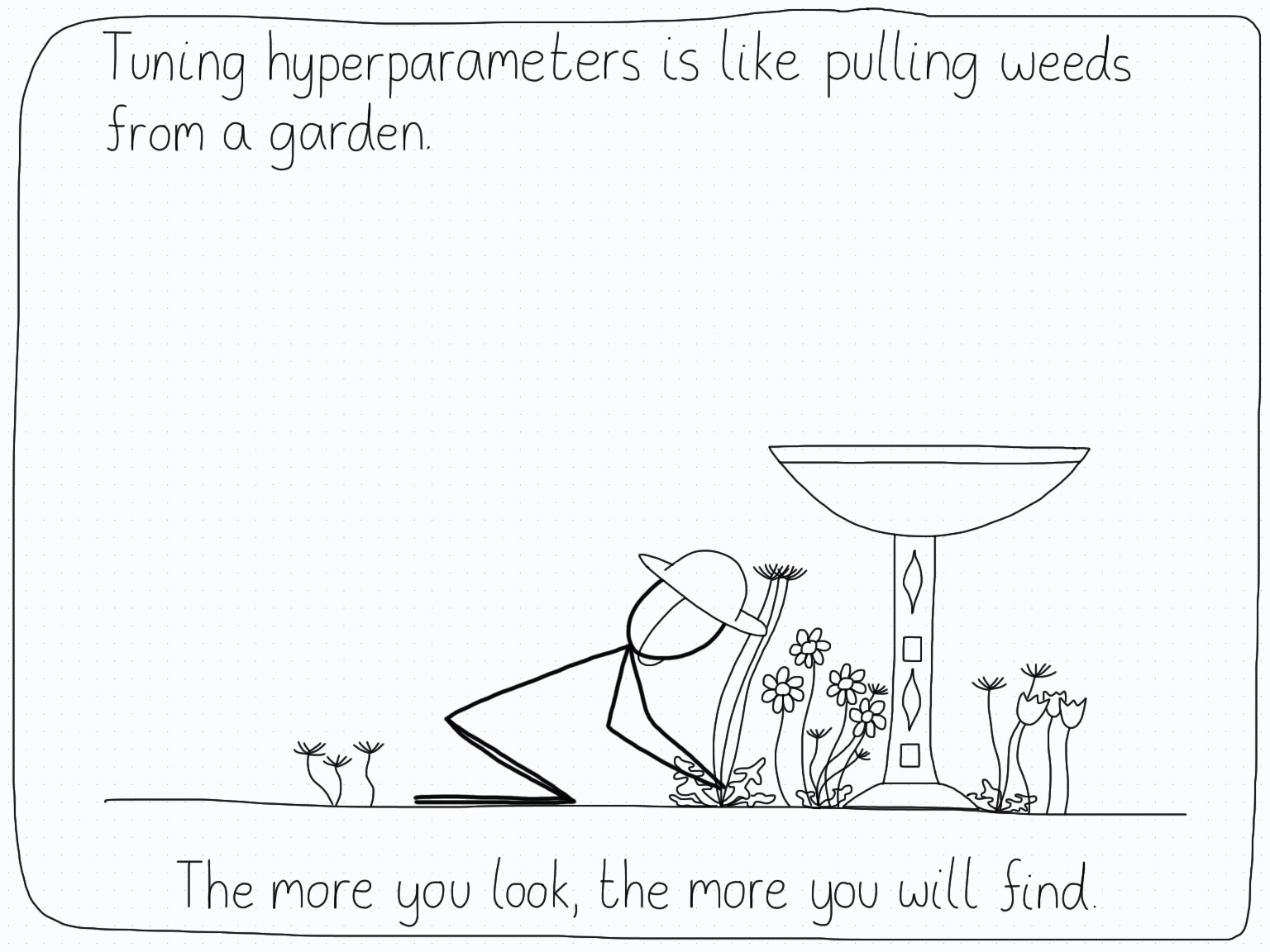
Those are just the hyperparameters that immediately come to mind. The thing about hyperparameters is that they are a little bit like weeds in a garden: the more you look, the more you find.
Some of these have a discrete number of options, while others (like the learning rate), can basically be any positive number. I think you can imagine where this is going. If you’re trying to find the optimal hyperparameters for your neural network, there are going to be a lot of combinations you can try. Because of the multiplication rule, the curse of dimensionality strikes again.
If we just look at the above hyperparameters, we’re already exploring a nine-dimensional space! Nine dimensions is a lot, which means searching through this space can be worse than looking for that needle in a haystack. At least with the haystack, we’ve limited ourselves to three dimensions.
In fact, while I thought the bulk of my project would involve coding the neural network, the real work was fiddling with the various hyperparameters, trying to see if I could squeeze out a bit more accuracy. This can be a frustrating endeavor, particularly when you’re working with a system whose performance you aren’t sure of. When should I give up with tuning and call the performance “good enough”? That’s the type of question I would ask myself. So by the time I was wondering if I was actually doing more tuning than the network itself!
It’s tempting to think that the neural network will do all the work for you, but that’s not true. The curse of dimensionality rears its ugly head again even for something as simple as getting a few model parameters adjusted.
Maybe you then have the clever idea of teaching another neural network to adjust those hyperparameters for you. While I imagine that could work, you’ve only kicked the problem down the road: How do you adjust the hyperparameters for that new neural network?
It’s turtles all the way down.
A flashlight in the dark
I once worked for a week on a problem at the intersection of quantum computing and machine learning. It was a project during my master’s degree that I did with two other students and some people from the company 1QBit. The idea was to explore the “loss landscape” of a quantum system to learn more about it (See Reference 4).
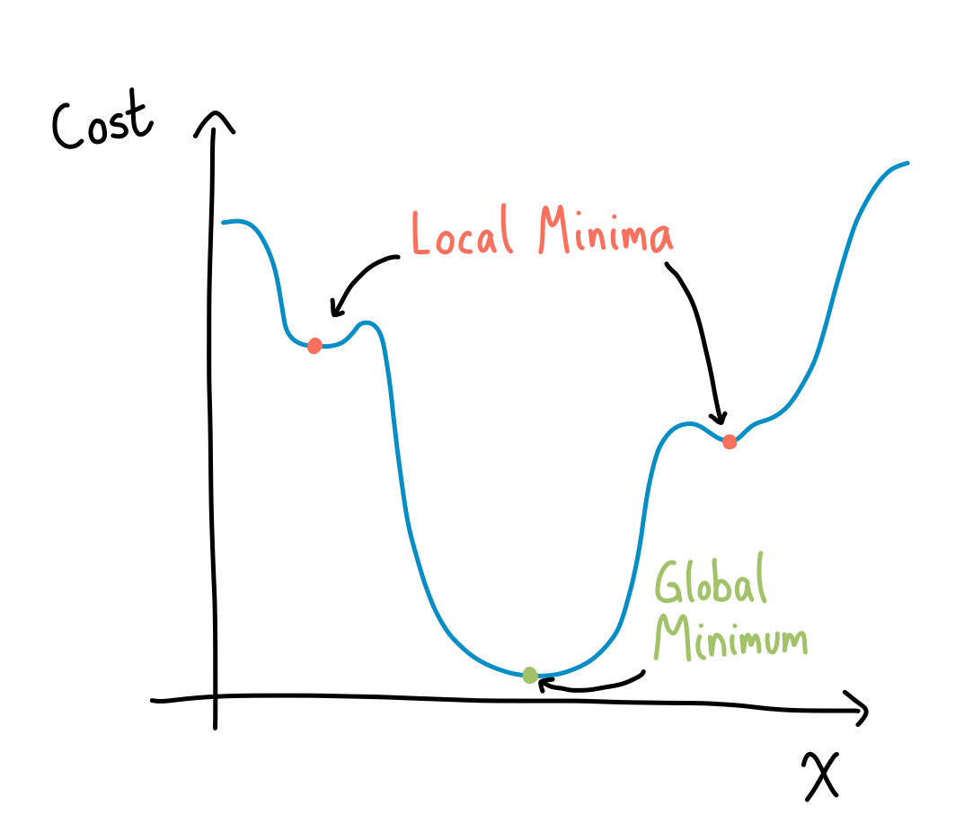
The loss landscape is an evocative name for something rather simple. When using some sort of gradient descent approach to a problem, there’s always a function you want to minimize. That function is called a “cost” or “loss” function. Minimizing the loss function means trying to find the local and global minima.
If we have a regular graph that we can visualize, seeing how we navigate to the minimum isn’t too difficult, like in the following example (note here that this means we only have one parameter, since the other is used to plot the cost).
We can even go up one dimension, where now we are looking at a surface and trying to find its minima. This is where the name “landscape” comes from. However, since these are difficult to draw, I will only show you an example of one from Pennylane’s post on barren landscapes (See Reference 5).

The tricky part is when you’re trying to minimize functions of many variables. The tools are the same (gradient descent or a similar procedure, find where the derivative vanishes, and check that it’s an actual minimum and not a saddle point), but the problem becomes more difficult. In higher dimensions, the landscape isn’t something we can visualize. Furthermore, there’s the added complication that higher-dimensional spaces are vast, which means finding solutions to your problem can be fraught with issues.
During the week I worked on this problem, I saw firsthand how having many parameters in a loss function can make it difficult to really understand the loss landscape of your model.
A blessing in disguise
From the examples I’ve talked about in this essay, it’s easy to take the mindset that the curse of dimensionality is all downside. However, it turns out that there’s a surprise waiting for us in higher dimensions.
Despite the difficulties we’ve seen, there’s also a complement to the curse of dimensionality: it’s sometimes called the “blessing of dimensionality”. To cap things off on a cheerful note, I want to dip our toes into how higher dimensions can work in our favour.
The rough idea is that going to higher dimensions can allow you to learn more about your data. This is relevant in statistics, where you want to do inference from the data. By accumulating more data, the different features (dimensions) you are considering become intertwined. This lets you “piggyback” on a connection between variables A and B to find out something about variable C, since it has a connection to B (See References 1 for the full example I described just above and 2 for more perspective on the blessing).
Befitting the month of October, the curse of dimensionality has the air of being a little scary. And for physicists like myself who study quantum many-body systems, it can definitely be a nuisance. But at the same time, encountering the complexity of the world can sometimes help, if we are willing to loosen the magnification of our lens and look at things a bit more fuzzily.
Just watch out for those high-dimensional loss landscapes.
References
- “A blessing of dimensionality often observed in high dimensional data sets”, by Jeff Leek.
This blog post gives a few examples of how doing statistics on many dimensions of data can be useful. I won’t pretend to know all of the details, but the point seems to be that high=dimensional data is helpful.
- “The blessing of dimensionality”, by Andrew Gelman.
This post talks about how not everything is bad about high-dimensional data. He makes the point that it can be a good thing as well, explaining the title.
- “Curse of Dimensionality”, Wikipedia. This page gives an overview of both the curse and the blessing, as well as some examples that are more mathematically-oriented.
- “Variational Circuits”, Xanadu. This post gives a nice idea to what I’m talking about. Basically, a quantum circuit with tunable parameters is built, and then you do machine learning to train the parameters of the circuit to fit the output you want (for us, it was the ground state of a Hamiltonian). The loss landscape is then the cost function you come up with to encourage the model to be tuned well.
- “Barren Plateaus”, Xanadu. This post shows an example of a barren plateau, which is very difficult for doing gradient descent. That’s because gradient descent and a lot of machine learning is based on the idea of taking derivatives and moving in the direction of most change (hopefully towards a minimum). A barren plateau is a region where the derivatives are almost zero everywhere, making it difficult to pick a direction.
Endnotes